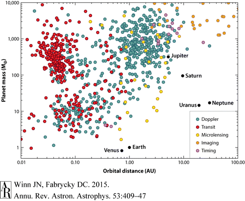
INTRODUCTION Background Throughout the history of exoplanet research there have been two main competing theories about how exoplanets form around their host stars. The first being a monistic theory, which suggests that planet formation is closely related to the formation of the host star, forming in the outer rings of the protostar. The dualistic theory, however, suggests that exoplanet and star formations are completely separate events, and that exoplanets either formed at a later time around the host star or that the exoplanets formed elsewhere and were captured by the host star. We will discuss the evidence that observers have collected over the years and give an overview of how the data can give us an insight on exoplanet formation. Since the first astronomers we have gradually come to know our own solar system well. We know that there are 8 planets, sorry Pluto, four being smaller and rocky and four being gaseous and larger in size. the orbits of it’s planets are very close to circular and have mean eccentricity of 0.06 and individual eccentricities ranging from 0.0068 to 0.21. Even the mean inclinations vary by only a little. We know this and more about our own solar system, but we don’t know if they are necessary for other systems to form, only that they may be clues to help discover them. Here we hope to add to our understanding of other systems. First we will review several different methods of exoplanet detection and the significance of each method. Each method has its own set of distinct properties that can help detect a variety of planets. Next we will discuss the geometry of exoplanet systems, regarding eccentricity and orbital distances, systems containing multiple planets and systems with multiple stars. The Kepler Missions - https://www.nasa.gov/mission_pages/kepler/overview/index.html https://www.nasa.gov/feature/ames/kepler/nasa-ends-attempts-to-fully-recover-kepler-spacecraft-potential-new-missions-considered https://ui.adsabs.harvard.edu/?#abs/2014PASP..126..398H A vast majority of exo-planet discoveries come from using the Kepler Space Telescope. Kepler is a 0.95 meter photometric telescope that orbits above Earth’s atmosphere. Its main goal is to find exoplanets, specifically Earth-like terrestrial planets that orbit in their host star’s habitable zone. Kepler’s first task was to explore over 150,000 stars in search of planets transiting in front of a star, which was a success. Early 2013 brought Kepler to the end of its first mission. Two gyroscopes used to carefully position the spacecraft had failed, and after several months of attempts to repair the craft NASA was forced to admit defeat. However, that was not the end of Kepler. Kepler can still work with just two working gyroscope wheels, by positioning the craft in the plane of the orbit it needs only the Y and Z axes wheels along with the X axis thrusters. Kepler takes continuous data while pointed at the same small portion of the sky, but must cycle through different fields of view during the year. This is due to having to avoid interference from the Sun, Kepler must reposition its target field of view roughly every 80 days so that the view is never blocked. To this day Kepler has discovered well over 2,000 exoplanets using the transit method of planet detection (NASA, 2017). METHODS Here we will delve into the the methods of detecting exoplanets. Each method has a selection bias in detection for planets with certain properties and therefore highlights the importance of having a diverse arsenal of detection methods. Figure 1 Giant planets dominate the observed systems even though small planets are more abundant when simulated. Hot Jupiter-like planets pile up in places, implying bias’ in our methods. Transit method http://iopscience.iop.org/article/10.1088/0004-637X/742/1/38/meta#apj404101s2 - done The transit method requires that planets be in the plane between our sight and the host star which clearly indicates a bias will form. Since this method measures light blocked by planets, it will tend to favor planets that have a larger mass and smaller orbital distance. Planets that are not in the line of sight will not be able to be detected, which is troubling when trying to get an accurate occurrence rate. To account for bias’ we factor in efficiencies, for the transit method they are the probability of the planetary orientation, the efficiency of the survey detecting the planets, and the rate of false positive events. These efficiencies will not remain constant, we must factor in the properties of the star as well as the properties of the planet such as radius and orbital period. The transit probability attempts to account for the random orientation of a planet around a host star. The probability is \eta_t_r = {a} = ({G\rho_*P^2})^{1/3} for $R \ll R_* with radius R*, semi-major axis a, and mean density ρ*. Here the mean density can be approximated as that of the sun for simplicity, as uncertainties will only affect the result as ρ−1/3. This equation implies that planets with higher eccentricity have a higher probability to be discovered. It should be noted that multi-planet systems do not have a different probability due to the fact that systems are randomly oriented . Discovery Efficiency - figure 2 — Dopplar Method The Dopplar method uses the Dopplar shift of the light received from stars and potential planets as a means of detection. Distinguishing these shifts in the light is extremely difficult due to the light noise from the host star, so the Dopplar method is ideal for large planets with a large orbital radius. Figure showing discoveries, page 4 The work done by has given some good insight on planet detection with the Dopplar velocity method. They observed nearly 600 stars searching for potential exo-planets for 8 years. They found that planets with very large masses and short periods were rare. Although, some candidates still need more time for detection, their data also shows that gas giants are about 5 times more likely to be detected with a period of 300 days or more, which differs from the theoretical predictions of a smooth increase in likelihood of gas giants forming the as the period increases. http://iopscience.iop.org/article/10.1086/588487/pdf - done In contrast, it has been found that small planets with short periods tend to occur in multiples around their host star. conducted a study in 2010 with a survey of almost 200 stars. Each star was taken to be well-defined, meaning each star had characteristics within a set of bounds that was deemed ideal for the survey including brightness, radial distance, luminosity, and observability. Taking several measurements of radial velocity over a five year span with the Keck Telescopes, they then matched the velocity measurements with the maximum planetary mass that would be possible given the velocity. For the stars where no planets were observed a calculation is done to determine a mass limit, above the limit we can determine that there is no planet possible with a high degree of certainty, below the limit we can not rule out the possibility of a planet. After accounting for the possible missed planets, they calculated the occurrence rate, focusing on the planets with a period of 50 days or less, and fit the data to a power law, {dlog{M_E}} = k*M_E^\alpha, where $k =0.39 $ and $\alpha = -0.48 $. Their results supported an occurrence rate of 1.2% for hot Jupiters within 0.1 AU, a rate of $14 \%$ for planets of 1 to 3 MEarth, and for Earth-like planets of 0.5 to 2 MEarth a rate of $23 \%$. Figure # Microlensing http://www.nature.com/nature/journal/v473/n7347/full/nature10092.html - done The microlensing method is much more effective than either of the previous methods for detecting planets at extreme distances. Unlike those methods, microlensing detections are based on the mass rather than luminosity, meaning that we don’t need to collect light from the planet or the light from the host star. This provides the ability to detect extremely far planets as well as ones that do not have host stars at all. The magnification is characterized by Einstien’s radius crossing time, t_E = {M_J}} days, where MJ is Jupiter’s mass, 9.5 × 10⁻⁴MSun. In 2007, with data from the Microlensing Observations in Astrophysics (MOA), several thousand microlensing events were observed. After narrowing the event down to about 500 that fit within their well defined criteria, the events were narrowed down to just 10 that had a tM of about 2 days. The Optical Gravitational Lensing Experiment (OGLE), another microlensing survey, was able to observe seven of those ten events and confirm six of the ten . Several features of exo-planet systems have been researched with several methods. We see that although there is some discrepency in the exact rate, gas giants tend to have long periods compared to small, rocky planets. SOLAR SYSTEM SHAPES Eccentricity The eccentricity of a planet gives it the shape of its orbit around its host star. An eccentricity of zero means that the orbit is perfectly circular and an eccentricity of one means the orbital shape is that of a parabola. Planets generally don’t have an eccentricity of one, however, as that would cause the planet to become detached from the host star’s gravitational pull and be sent of into space. http://www.aanda.org/articles/aa/pdf/2004/35/aa1213.pdf - STARS - done here used the data of the The Ninth Catalogue of Spectroscopic Binary Orbits (SB9) to try to show a correlation between a planet’s period and eccentricity. The catalog adds to the previous edition published three years prior and shows data up to May of 2004. SB9 contains data from 2386 systems. http://www.aanda.org/articles/aa/pdf/2001/32/aade293.pdf - done. here conducted a study on the highest eccentricity planet known at the time, HD 80606. With an eccentricity of 0.927 and mass of 3.9MJup. formulated several ideas on the cause of the abnormally high eccentricity. First, the eccentricity could be due to interactions between the planet and a disk, however, a recent study suggests that this would only happen for objects with a much higher mass such as a brown dwarf. Another possible cause would be interactions with other planetary objects. Certain dynamical instabilities could lead to this high eccentricity and even eject a planet out of the system all together. http://iopscience.iop.org/article/10.1086/590047/pdf - done builds on the latter theory by running simulations of forming solar systems. They used two different computer clusters to run their simulations, one for short-lived systems spanning about 10⁶ years and one for longer-lived systems spanning from 10⁶ years to 10⁸ years. The initial conditions for semimajor axis and planetary masses were chosen from a larger, but reasonable distribution. The initial number of planets were chosen to be 3, 10, and 50 for different runs. Planets were made to be homogeneous spheres with densities of 1g × cm−3. In all but one run the planets were allowed to collide and assumed to be inelastic. They make several, admittedly “aggressive”, interpretations of the final results. First, they discuss the early stage of the formation process, where the initial conditions are determined before the simulations run. Quite plainly they state that there may not be a "good’ set of initial conditions and that the conditions might be much more random than previously thought. It is also mentioned that the systems before the simulation actually runs must be dynamically active themselves. Next, planet to planet interactions do change the planes of the planets, widening the distributions of inclinations. The average number of planets in a system should be 2 to 3 after a period of 10⁸ years, regardless of the number of initial planets at the beginning of the simulation. Just 5% of systems had four or more planets. This suggests that if one exoplanet is detected in a system, it is likely that to host at least one other similar planet. For e ≥ 0.2 the final results of the simulations agree very well with observed eccentricities of exoplanet solar systems. The results also showed a deficiency of planets with e ≤ 0.2, which might suggest that the population of systems is not dynamically active or that there is a dampening of the eccentricities due to gas and other planetesimals. Observation tells us that only about a quarter of exoplanet systems are inactive. They found that there was also very little correlation with semimajor axis distance and eccentricity. The Roche Limit - http://iopscience.iop.org/article/10.1088/2041-8205/773/1/L15?fromSearchPage=true - done The Roche Limit is the distance at which an object that is held together by means of its own gravity will experience tidal force from a second object that will cause the first object to be destroyed. As one can see, the limit clearly plays a significant role in determining how close a planet can safely orbit a host star. The Roche Limit can be expressed by, d = 1.26R_m (\dfrac {\rho_M}{\rho_m})^{1/3} where RM is the radius of the secondary object, ρM is the primary object density, and ρm is the secondary object density. The density ratio is a defining factor of the limit just by inspection. A study by reinforces this by examining the planet with the shortest known orbit, 4.2 hours. Assuming an iron core and silicon mantle they find a planetary density between 3.5 - 3.9 g/cm and 10-12 g/cm. This leads to a possible period of 3.6 hours and 6.0 hours respectively. Transit Eccentricities - http://iopscience.iop.org/article/10.1088/0004-637X/756/2/122/pdf - done http://iopscience.iop.org/article/10.1086/522039#pasp_119_859_986s2 - done The vast majority of our knowledge on eccentricities in other solar systems comes from the Dopplar detection method. The transit method can not directly tell us a planet’s eccentricity as the velocity measurements are difficult to determine due to the faint images. takes a particular interest in investigating the eccentricities of hot Jupiters, planets that are so close to their host star that they couldn’t have formed there. The main theory of how these kinds of planets came to be in such a close vicinity to their star is that they were moved there by gravitational perturbations with other celestial objects. Therefore these kinds of planets should show up as failed and partially formed as well as complete planets as the perturbations may have taken place at any point in the planet’s formation cycle. shows that the eccentricity of a transiting planet can be accurately measured by using a light curve. They demonstrated by using a planet with a known eccentricity, HD 17156 b with an e = 0.67 ± 0.08, and fit it with with a few simulated light curves using data from both partial and full transit observations. Barnes describes the process, first create light curves using some assumed data about the planet such as as the period if the eccentricity were zero as well as a best fit light curve. The eccentricity induces varying planetary velocities throughout it’s orbit and those variations will show as asymmetries on the best fit light curve. The two can then be compared to determine the eccentricity. Barnes also makes an important note that this will not work with very small eccentricities as the small effect likely will not show on the light curve. The main takeaway from these paper is that light curves from transit observations can give reasonably accurate estimate of a planet’s eccentricity. The highlight being that this light curve method does not require radial velocity measurements, which often can not be measured due to the faintness. Furthermore, exoplanets that are bright enough for radial velocity measurement will benefit with more precise eccentricity measurements with more accurate constraints. SYSTEMS WITH MULTIPLE EXO-PLANETS http://iopscience.iop.org/article/10.1088/2041-8205/732/2/L24/meta;jsessionid=D451DE8A7E27BCE57FDB4839725F2BCE.c1.iopscience.cld.iop.org Inclinations Are coplanar planets normal? Intro https://academic.oup.com/mnras/article-lookup/doi/10.1093/mnras/stt1657 There are some planets that orbit with an irregular inclinations, however, the majority of the discovered planets share an inclination with their star’s disk remnant. This does not necessarily mean that the systems formed that way, their inclinations may have changed due to various purterbations after the system’s formation. Given a monistic theory of planet formation, planets should form coplanarly in a single disk of gas. makes this simple but powerful theorization. discusses one system in particular, HD 82943, a Sun-like star with that hosts two Jupiter-like planets at roughly 1 AU. Recent data has shown that the inclination of orbit for these two planets is 20 deg +- 4 deg. It must be assumed that these planets share the same inclination, else no constraints can be made on the inclination. The evidence also shows that the star has an inclination of 28 deg +- 4 deg. This implies that there is an extreme likelihood that HD 82943 and it’s two planets have the same or nearly the same inclination. Gravitational Scattering - http://www.sciencedirect.com/science/article/pii/S0019103504002106 - done The planets in our own Solar System travel on roughly the same coplanar inclination around the Sun, however, there is nothing that says we can not have systems of planets that have varied inclinations of orbits. This suggests that the closeness of inclination is related to the initial conditions of the formation of the Solar System. It is possible that systems of highly inclined planets are prevalent, but instabilities in the obits cause a number of the planets to collide or otherwise be destroyed. investigates and discusses how exoplanet systems form with respect to their inclination. We just can’t know if these systems formed in the same plane together or if they formed in a system with high inclinations. They explain that there are some cases where known multiple planet systems where some constraints can be put on the systems, but these only rule out extreme variations in the systems. They also acknowledge that gravitational scatter from planet to planet could play a key role in high inclination planets and to a lesser extent, eccentricities. While scattering inward is an unlikely explanation for hot Jupiters, it is a very plausible theory to explain outward scattering given observations of stellar disk debris. Large radii would be fairly common for these planets, accompanied by higher eccentricities. finally discusses that the calculations done as well as the overall prediction is consistent with our observations of exoplanetary systems. However, gravitational scatter would take place on a shorter scale than the typical timescale of disk dissipation. This tells us that there must be some other forces that come into forming a planet’s inclination and eccentricity. The formation of planets with relatively large separations would lack this gravitational scattering and be subject to lower amounts of dynamical changes. If the separations were random, then only a fraction of the systems would be subject to the scattering, which is the case given past observations. This leads to the conclusion that planet to planet gravitational scattering as well as disk-driven migration share a part in planetary system formation. Planetary Spacing http://ac.els-cdn.com/S0019103598959991/1-s2.0-S0019103598959991-main.pdf?_tid=4c95fd90-292d-11e7-ad71-00000aab0f6b&acdnat=1493066199_8aa595230cea7e606a36ed49b4590303 The Titius-Bode Law can accurately predict the orbital spacing of every planet in our own Solar system, with the exception of Neptune. This law, an = 0.4 + 0.3 × 2n in AU, not only works for our eight well known planets, but also predicts Ceres and the asteroid belt. The dwarf planet Pluto also fits well into the series if Neptune were excluded. So does Bode’s Law only apply to our system of planets or is there more to it? Simple simulations can be used to test Bode’s Law. First, we must make a few constraints. Planets should not be stable in their orbits with respect to other planets, in otherwords, they need to be a sufficient distance way in order to avoid instabilities. Results of the simulation will be highly dependent on the distances that are determined to meet those conditions. The simulations are run, running several thousand times per conditions that need to be met. Some exceptions are allowed to be made in these simulations, mirroring the exceptions that are often made to Bode’s Law when it concerns the Solar System. A gap in the models is also allowed to take place, as it does in the Solar System in the form of the asteroid belt. From the data concludes that with stricter conditions on the radii, the systems tend to fit better with Bode’s Law. With no exceptions or gaps, the Solar System doesn’t fit much better than near random simulations that have very relaxed conditions. With gaps and up to three exception planets allowed, the Solar System fits very well. However, these exceptions were made specificly to make it fit better to Bode’s Law. admits that the approach used is very simplistic, if simulations were to be done with realistic orbit integrations instead of random ones then the results would likely fit a general Bode Law much better. https://academic.oup.com/mnras/article-lookup/doi/10.1093/mnras/114.2.232 - done Another aspect of this to be considered deals with mean motions and resonance. Using data taken from Connaissance des Temps in 1949, the goal of was to find every resonance between two bodies in the Solar System up to an arbitrary upper limit of 7. With this they could determine the frequency of resonances with respect to random planetary spacings. ϵ was defined as a degree of commensurability, which compared the actual resonance with theoretical resonances. It can be represented by, \epsilon = \lvert {n_1} - {A_1} \lvert where n₁ ≤ n₂. A₁ and A₂ are both integers up to 7 and A₁ ≥ A₂. From here we can find any resonances between celestial bodies. Each of the eight planets as well as Pluto share several resonances with each other. Furthermore, in a sample of 46 pairs, several moons of the Solar System share resonances, one with the two moons of Mars, seven within the moons of Jupiter, 16 within the moons of Saturn, and 9 within the moons of Uranus. Next, calculating the probabilities of the resonances of the Solar System and of a control distribution of moons with resonances. finds that the universe has some preference toward resonances, as there is a much lower chance of finding planets and moons with these spacing and resonances than if by random chance. PLANETS IN BINARY STAR SYSTEMS With the more recent discoveries of exoplanetary systems, the question of whether binary systems can also form planets has become increasingly of interest. The notion of binary systems is nothing knew to us, they can be comprised of anything from white dwarfs to main sequence stars like the Sun to black holes. The majority of current models of planet formation use only one star, a bias that stems from our own solar system We will examine how the addition of a second star would likely affect the formation of planets in it’s system. http://www.aanda.org/articles/aa/pdf/2012/06/aa18051-11.pdf - done S-TYPE ORBITS https://arxiv.org/pdf/1406.1357.pdf - done http://www.aanda.org/articles/aa/pdf/2009/04/aa10639-08.pdf - 2009 1st - done http://iopscience.iop.org/article/10.1086/504823 - 2006 2nd - done S-type orbits are systems in which the planet orbits one of the two stars in the system, gives an occurrence rate of at least 12% for S-type orbit exoplanet host systems based on the most recent Extrasolar Planets Encyclopedia. Prior to this, it was calculated to be 17% and 23% by and , respectively. discusses how the formation of S-type planets can be altered as the accretion disk develops. From observation, formation disks are less frequent and less massive compared to single stellar systems. This especially applies to close orbit stars, at a separation distance of 40AU or less. Extreme cases can cause disks to have insufficient gas and dust to form planets. Furthermore, accretion in multi-star systems can be accelerated, giving a much lower timescale in which planets can form. https://arxiv.org/pdf/0806.0819.pdf - done In the intermediate stages, planetesimals would form and increase in size through impacting one another. This would happen at an increasing rate, requiring very few perturbations. The key is the low impact velocity required for planetesimals to combine, which is lower than their escape velocity. The gaseous disk causes as drag force on the developing planetesimals, which is size dependent and causes different orbits depending on the size of the object. The larger of the planetesimals tend to have less stable orbits and are prone to oscillations inside the disk. The addition of a second star, however, will slow the velocity of the orbiting objects and dampens their growth. This in turn makes planet formation difficult, which is exactly what found while studying the systems of α Centauri A and B when they simulated planet formation. It is noted that it is much more probable that planets could form very near the host star as the effects of the binary system would be much less in regions around 0.5 AU. http://iopscience.iop.org/article/10.1088/0004-637X/791/2/111/pdf - done A majority of planets found to be in multiple star systems we found before the second star of the binary system. Once a planets have been detected via Kepler with the transit method, another search is then conducted using Dopplar and direct imaging. In a study that uses this exact method it is found that the occurrence rate for multiple star systems is different from that of single star systems . For binary systems with less than 1500AU separation distance there is less than a 50% chance on average of finding planets than in single and the probability decreases as the distance from the star decreases. Once the separation distance exceeds 1500 AU the difference in occurrence rate is negligible, therefore the binary system likely a very small effect on planet formation. P-TYPE ORBITS P-type orbits also involve a system of two orbiting stars, however, instead of a planet orbiting a single star the planet orbits both. P-type orbits are seem to be rarer than S-type orbits, Kepler has so far found several P-type orbit planets, though they seem very rare compared to S-type. It is difficult to get an idea of the occurrence rates for these types of planets. All P-type orbits have been found to be greater than 3 Earth radii. It is thought that this is due to the fact that these planets would be very hard to detect rather than smaller radii being devoid of planets . CONCLUSION The study of exoplanets is still relatively new in the field of astronomy, though we are quickly making leaps and bounds in our research. We have developed and supported a monistic Solar System formation theory and have made countless observations of it in hopes to apply them to systems beyond our own. Detection methods such as the transit method using the Keplar Space Telescope have been crucial to extending our understanding of exoplanets. It is of paramount importance that we have several methods of detection, not only to avoid as much bias as possible, but so that we can continue to improve upon the data and discoveries that we make everyday. Orbital eccentricity and inclination both play a major role in the architecture of exoplanetary systems. The focus needs to be on what happens before the formation of planets, as well as during and after. Interactions in these need to be heavily considered in formation theory. The methodology behind discovering both are just as important, if not more important as it can tell us how these systems came to be. Even simplistic models shed light on the creation of said systems, including our own, and can fit our monistic model. From there we can revise and retest our theories and refit our data. Many of the papers and studies mentioned here are still in the early stages. Data is still being collected, Keplar for example is still searching for more exoplanet systems and will be for as long as it lasts. We are by no means done simulating eccentricies or inclinations and we are far from having difinitive proof of how planets form in binary systems. This is encouraging and despite having made a numerous amount of progress already, there is still much, much more to go.


/ProductionFCN32_SuitAppIFCN8_confusion (copy).png?1493888536)