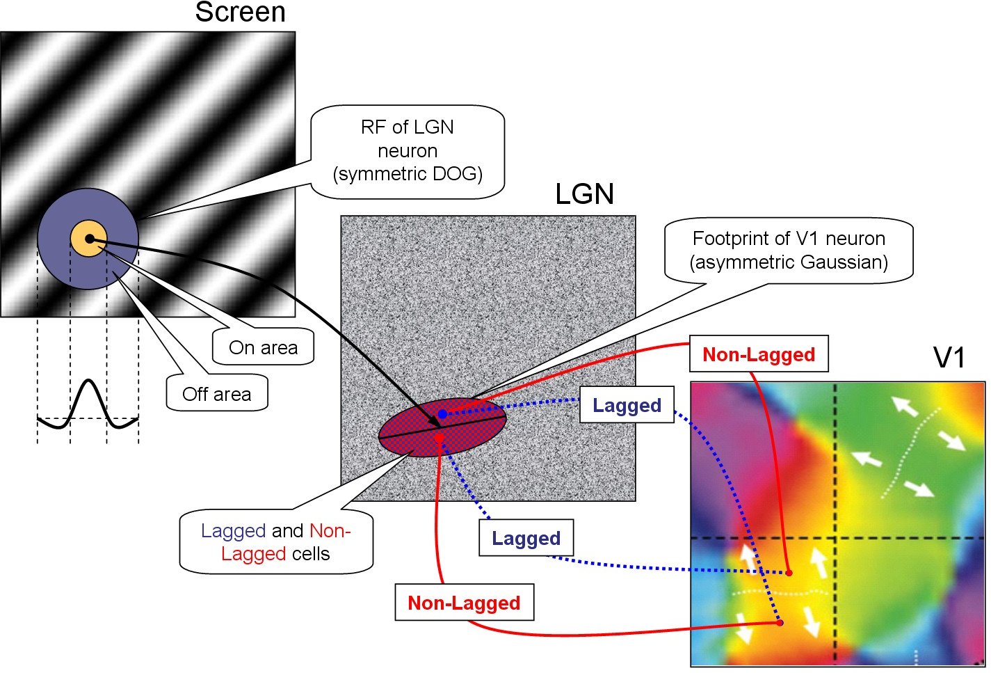
INTRODUCTION Primary visual cortex neurons are selective to various characteristics of the stimulus: orientation, direction of motion, color, etc. [14]. Up to now, some important questions about the underlying mechanisms of these properties remain unanswered. Mathematical modeling is a perspective method of the V1 studies. In our previous works it was developed a biophysically detailed V1 model that reflects orientation tuning [11], [8]. Here we develop this model, supplying it with direction selectivity. Direction-selective (DS) neurons exist in almost all animals that have a visual apparatus. Principal DS models (Hassenstein-Reichardt model, Barlow-Levick model and fully opponent Hassenstein-Reichardt model) are well known and discussed in [3]. Most of the DS models include a time delay between the spatially shifted inputs in cortical cell [1-2]. There is an important question about the source of the time delay. The physiological mechanism of this delay formation is disclosed in experimental work [4] and in more details in [24], where with the help of intracellular _in vivo_ registration it was demonstrated that LGN neurons fall into two classes of lagged and non-lagged cells, and the delay is determined by the effects of the inhibitory-excitatory synaptic complexes formed on synaptic axonal terminals of retinal ganglion cells in LGN. In the papers [17], [23], it was proposed a complex schematic model of DS, on a basis of a specific convergent projections of the signals from LGN cells with and without a delay and intracortical interactions. The temporal difference and the structure of LGN inputs provides DS in V1. We have taken into account these mechanisms to reproduce DS in our biophysically detailed visual cortex model. METHODS Lagged and non-lagged cell based mechanism of DS A simple scheme of the proposed model is presented in Figure 1. The model reproduces the direction selectivity in V1, in response to moving gratings. The model contains three two-dimensional levels: the screen with moving gratings (left panel); LGN (central panel) consisted of neurons with the center-surround receptive field (RF); V1 (right panel) consisted of neurons with more sophisticated RF. The center-surround RF structure is typically described as a difference of Gaussian functions. An example of the LGN neuron’s RF is shown in Fig. 1 (on the left). There are two types of LGN cells – lagged (with time delay 30 μs) and non-lagged (without delay). At the level of V1, neurons are organized into orientation hypercolumns, and the model was constructed so that the neurons of neighboring hypercolumns would prefer opposite directions of movement. The details of the model which provides DS in V1 are as follows. V1 neurons receive inputs from LGN cells which are located within the footprint described by asymmetric Gaussian. The neurons of two neighboring hypercolumns preferring the same orientation but opposite directions have the same footprint. The difference of preferred directions is provided by the following property of input. The footprint is splitted along more elongated axis into two halves. V1 neurons preferring one direction get input signal from non-lagged cells located in one (right) side of the footprint and from lagged cells located in the other (left) side, whereas V1 neurons preferring the opposite (downward) direction conversely get input signal from non-lagged of the second (left) side and from lagged of the first (right) side. Stimulus Presented stimulus is a moving gradient characterised by the orientation, spatial frequency and temporal frequency. LGN Neurons in LGN display a center-surround receptive field (RF) structure, responding most strongly to visual input in the center of a specific location of the visual field and being inhibited by visual input in the surround. This center-surround RF structure is typically described as a difference of Gaussians (see [12] eq. 2.46). The spatial and temporal aspects of RF are usually assumed to be independent. We describe the temporal component by a function as in [12], eq. 2.47, but add a coefficient controlling the balance between early and late components of LGN cell response. The firing rate of an LGN neuron at any given time is expressed as a convolution of RF with the stimulus, eq. 2.1 in [12], rectified then by a non-linear function which zeroed the firing rate if the convolution is negative. The model of LGN cells is described in detail in [25]. V1 Neurons in V1 show more complex RFs than LGN cells and respond vigorously to moving (or steady) oriented gratings within their RFs. We assume all neurons in V1 to be tuned to direction, in spite of the fact that some neurons are tuned only to orientation [15]. The model of V1 is based on the CBRD model describing orientation processing [11]. V1 is modeled as a continuum in 2-dimensional space along the cortical surface. Each point of the continuum contains 2 populations of one-type’s neurons, excitatory and inhibitory. The populations are interconnected by synapses of AMPA, NMDA and GABA types and have AMPA- and NMDA-synapses formed by external axons. The strengths of the external connections are distributed according to a pinwheel architecture, thus neurons receive inputs according to their orientation and direction preferences. The strengths of the intracortical connections, the maximum conductances, are distributed according to the locations of pre- and postsynaptic populations. The most strong connections are local and isotropic, thus depending only on the distance between the pre- and postsynaptic populations and decaying with the distance. Patchy long-distance connections are also taken into account, but they are much weaker. Within one population located at a given point the neurons receive the common inputs from presynaptic populations and an individual noise. The membrane potentials and ionic channel states of these neurons are dispersed due to the noise, being rather distributed in a space of neuron refractority characterized by a time passed since the last spike of each neuron. Neurons with the voltages crossing a spike threshold contribute into the population firing rate, which is the output characteristic of the population activity. According to the structure of connections described above, the firing rate determines the presynaptic firing rate, which, in turn, controls the dynamics of synaptic conductances. The presynaptic firing rate pre-determined by the excitatory population firing rate determines the dynamics of AMPA and NMDA synaptic conductance, the inhibitory one controls GABA conductance. The synaptic conductances are the inputs for the postsynaptic neuronal populations. Subjected to the electrotonic effect provided by the dendritic compartment, the membrane voltage distribution across the refractory time space is controlled by the synaptic conductances. Again, it determines the output firing rate and so on. The external presynaptic firing rate is distributed according to retinotopic projection. The orientation preferences are set by the pinwheel architecture. The pinwheels with clockwise progression of orientation columns are adjacent to the ones with counterclockwise progression. The pinwheel-centers are distributed on the rectangular grid with the pinwheel radius R and indexed by iPW and jPW. The adjacent columns owing to different pinwheels have the same orientation preferences. The coordinates of the pinwheel-center are xPW = (2 iPW − 1)R, yPW = (2 jPW − 1)R. The orientation angle for the point (x, y) of V1 which belongs to the pinwheel (iPW, jPW) is defined as θ(x, y)=arctan((y − yPW)/(x − xPW)). The progression is determined by the factor ( − 1)iPW + jPW. Finally, the input firing rate is \varphi _{Th\; E} (x,y,t)=\iint dd\, D^{LGN-V1} (x,y,,)\, L_{LGN} (,,t-\delta(x,y,,)) , where $D^{LGN-V1} (x,y,,)={\pi \; \sigma _{pref} \sigma _{orth} } \exp \left(- }{\sigma _{pref}^{2} } - }{\sigma _{orth}^{2} } \right)$, where LLGN is the activity of the non-lagged LGN neurons at ($,$), (xcf, ycf) are the coordinates of the centre of the footprint of V1 neuron in LGN, xcf = xcf(x, y), ycf = ycf(x, y); δ is the delay of activity of the lagged neurons. The direction preferences are given by a combination of inputs from lagged and non-lagged LGN neurons: L_{LGN} &&(,,t-\delta(x,y,,)) \approx \nonumber \\ &&\left[L_{LGN} (,,t)-\delta(x,y,,) (,,t)}{\partial t} \right]_{+} \delta(x,y,,)=30~ms\quad \quad (-1)^{i_{PW} +j_{PW} } x'>0; \quad 0, \quad , x'=(-x_{cf} )\cos \theta -(-y_{cf} )\sin \theta , y'=(-x_{cf} )\sin \theta +(-y_{cf} )\cos \theta . The mathematical description of each population is based on the probability density approach, namely, the conductance-based refractory density (CBRD) approach [5-7], where the neurons within each population are distributed according to their phase variable, the time elapsed since their last spikes, $\ts$. The CBRD for adaptive regular spiking pyramidal cells and fast spiking interneurons is given in [11]. The model of an excitatory neuron takes into account a set of voltage-gated ionic currents. It is based on the CA1 pyramidal cell model from [13], where instead of full description of calcium dynamics and calcium-dependent potassium currents the cumulative after-hyperpolarization (AHP) current has been introduced according to the work [16], which provides the effect of slow spike adaptation. The inhibitory synapses are assumed to be located at soma, whereas the excitatory synapses are at dendrites. As the synaptic conductances are usually measured at soma, the two-compartment model from [10, 11] implicitly solves the reverse voltage-clamp problem, estimating the dendritic synaptic current. To describe the synaptic AMPA, GABA and NMDA dynamics the second order ordinary differential equations for the non-dimensional synaptic conductances were used, see [9]. The input function to these equations are the presynaptic firing rate. The calculations of presynaptic firing rates for horizontal connections are presented in [11], whereas the presynaptic thalamic input has been modified as described above. The basic parameters are given in [11]. The specific parameters of our simulation as as follows. Synaptic parameters: $_{ampa\; Th\; E} =0.4$ mS/cm, $_{ampa\; E\; E} =0.4$ mS/cm, $_{ampa\; E\; I} =0.4$ mS/cm, $_{gaba\; I\; E} =0.8$ mS/cm, $_{gaba\; I\; I} =0.2$ mS/cm, $_{nmda\; Th\; E} =1.6$ mS/cm, $_{nmda\; E\; E} =1.6$ mS/cm, $_{nmda\; E\; I} =1.6$ mS/cm, τrAMPA = 1.7ms, τdAMPA = 8.3 ms, τrGABA = 0.5 ms, τdGABA = 20 ms, τrNMDA = 6.7 ms, τdNMDA = 100 ms, Mg = 2 mM, VAMPA = VNMDA = 0, VGABA = −77 mV. Region geometry: cortex region is 1 mm x 1.5 mm, containing 2x3 regularly distributed pinwheels. Numerical parameters: time step 0.1ms, spatial grid 24x36, the $\ts$-space was limited to 100 ms and discretized by 100 points. RESULTS The constructed model proposes the detailed, conductance-based description of neuronal population activity in V1 and simple, filter-based description of retino-thalamic visual signal processing. The generalized model keeps the advantages of the former model [11] to relate different experimental observations obtained in slices and in vivo in visual cortex and allows us to consider experiments with moving stimuli. Here we verify by simulations (Fig.2) that the mechanism based on asymmetrical projections of lagged and non-lagged thalamic neurons to the cortex does allow the biophysical model to reproduce the direction selectivity in an extent consistent with experimental evidences, e.g. [19]. Also, we consider effects of surround suppression, stimulus locking, apparent motion and divisive normalization. Directional selectivity In our numerical experiments we presented moving gratings and reproduced the visual cortex activity. The modeled area of the cortex was as large as 1mm x 1.5mm and included 6 orientation hypercolumns. Spatio-temporal distribution of neuronal firing activity reveals the tuning of neurons to the direction of grating movement. As seen in Fig.2, the spike response of a neuron to the preferred and non-preferred directed stimuli were different (compare bottom plots in Fig.2C and D). This excitatory neuron located in the orientation column that prefers horizontal orientation. Its preferred direction is upward. A nearby neuron of the neighbor, lower orientation hyper-column prefers opposite direction (traces are not shown). Such tuning is provided by the cumulative effects of the described in Section 2.4 projection of LGN to V1 (Fig.1), the threshold rectification in V1 neurons and the recurrent intracortical inter-actions. Indeed, the light intensity was the same for the both stimuli (top frames in Fig.2A,B and top plots in Fig.2C,D). According to the model construction, the signal in LGN is not tuned (not shown) but its projection to V1 excitatory neurons is tuned (compare second to bottom plots in Fig.2C and D). The mean membrane voltage of the excitatory neurons is even more tuned (compare third to bottom plots in Fig.2C and D), which is due to the effect of recurrent synaptic inputs (forth to bottom plots in Fig.2C and D). The inhibitory interneuronal activity is reflected in the GABAergic conductance at the excitatory neurons. The threshold rectification producing the firing rate (fifth to bottom plots in Fig.2C and D) sharpens the voltage. The firing rate determines the probability for a single neuron of a population to generate spikes. With known synaptic conductances, a behavior of a single representative neuron is recon-structed and shown in bottom plots of Fig.2C and D. Stimulus locking The effect of long response to short stimulus called here as stimulus locking is the most challenging. It observed in experiments in cats and monkey . The response to 50 ms-spot of light lasts as long as 300 ms. At the same time, it is not trivial to find such long characteristic time scale in the mechanisms involved in generation of the response, except the adaptation which should lead rather to damping than prolongation of the response. However, our model is able to reproduce the effect ([Fig_SL], bottom trace). We have found that the most critical factor for this effect is the recurrent excitation. The effect was observed for the $_{ampa\; E\; I}$ from the range of 0.4 ÷ 0.5 mS/cm². The mechanism might be explained with the vector plot ([Fig_VectorPlot]). For the particular parameters chosen, the tuning of the cortical excitability is characterized with a basin of slow change of states in the phase plot of νE, νI (green bounded region). A stimulus abruptly shifts the state of the system from low rates (left bottom point) to high rates (right top point). Then the system gradually travels from this point down to the initial state (orange dotted line). Because the trajectory goes through the low change rate basin, the excitatory and inhibitory firing rates change slowly in the interval between 100 and 300 ms, as seen in Fig.[Fig_SL]. Apparent motion The stimulus locking effect allows the cortex to keep excitation for a while and thus link the stimulus with the following stimuli. In particular, this property is expressed in apparent motion, which can be observed, for example, if compare the activity in response to a moving spot (Fig.[Fig_MovSpot]) with that to a jumping spot (Fig.[Fig_3Spots]). The responses are similar in the sense that the focus of activity gradually travels from one cite to another without jumps. Surround suppression The surround suppression is revealed in experiments with different size stimuli. The response of the cortex non-monotonically depends on stimulus size [Rubin et al. 2015], such that the amplitude of the response to a larger stimulus might occur smaller than that to smaller stimulus. It is reproduced in our model (Fig.[Fig_SS]). Divisive normalization Sharpening by saccades As observed in , saccades increase the precision of the cortical response to stimulus. We reproduce the effect in simulations, as seen in comparison of Fig.[Fig_Saccades] with Fig.[Fig_noSaccades]. High amplitude bursts of the excitatory firing rate occur after rapid change of the “eye” position (Fig.[Fig_XYsaccades]), if the new position corresponds to bright stripe of the gratings. DISCUSSION We have introduced the direction selectivity in the model by implying the existence of a direction selectivity map, however such map is not observed in all animals. It is present in rabbits and ferrets. In monkeys, the directional map is absent in V1 but present in V2 [18]. With or without maps in V1, DS is a common feature of visual cortex neurons for various animals. It is quite possible that the mechanism of DS in animals without the directional map is similar to the mechanism in animals with such a map, like the one implemented in our model. The main mechanism of DS, according to our model, is the same as in the principle Hassenstein-Reichardt model based on the delayed excitation. Namely, the time delay between lagged and non-lagged neurons of LGN provides DS in V1 neurons. At the same time, Barlow-Levick mechanism also contributes to the direction tuning in V1 neurons because of the intracortical inhibition that is taken into account in our model. Concluding, the proposed model might be recommended as a tool to systematize various experimental observations focused to study mechanisms of the primary vision. ACKNOWLEDGEMENTS This work was supported by Grant No. 15-04-06234a from the Russian Foundation for Basic Research to AVC. REFERENCES 1. Adelson, E.H., Bergen, J.R.: Spatiotemporal energy models for the perception of motion. J. Opt. Soc. Am. A. 2, 284–299 (1985) 2. Barlow, H.B., Levick, W.R.: The mechanism of directionally selective units in the rabbit’s retina. J. Physiol. (Lond.). 178, 477–504 (1965) 3. Borst A., Helmstaedter M.: Common circuit design in fly and mammalian motion vision. Nat Neurosci. 18(8), 1067-1076 (2015) 4. Cai D., DeAngelis G.C., Freeman R.D.: Spatiotemporal receptive field organization in the lateral geniculate nucleus of cats and kittens. J. Neurophysiol. 78(2), 1045-1061 (1997) 5. Chizhov A.V., Graham L.J., Turbin A.A.: Simulation of neural population dynamics with a refractory density approach and a conductance-based threshold neuron model. Neuro-computing. 70(1), 252-262 (2006) 6. Chizhov A.V., Graham L.J.: Efficient evaluation of neuron populations receiving colored-noise current based on a refractory density method. Phys. Rev. E 77, 011910. (2008) 7. Chizhov A.V., Graham L.J.: Population model of hippocampal pyramidal neurons, linking a refractory density approach to conductance-based neurons. Phys. Rev. E 75, 011924 (2007) 8. Chizhov A.V., Smirnova E.Y., Graham L.J.: Mapping between V1 models of orientation selectivity: From a distributed multi-population conductance-based refractory density model to a firing-rate ring model. BMC Neuroscience. 10, 181 (2009) 9. Chizhov A.V.: A model for evoked activity of hippocampal neuronal population (in Rus-sian). Biofizika. 47(6), 1086-1094 (2002) 10. Chizhov A.V.: A two-compartment model for the dependence of a postsynaptic potential on a postsynaptic current, measured by the patch-clamp method (in Russian). Biofizika. 49(5), 877-880 (2004) 11. Chizhov A.V.: Conductance-based refractory density model of primary visual cortex. J. Comput. Neurosci. 36, 297–319 (2014) 12. Dayan P., Abbott L.F.: Theoretical Neuroscience: Computational And Mathematical Mod-eling of Neural Systems. The MIT Press (2001) 13. Graham L.J.: Interpretations of Data and Mechanisms for Hippocampal Pyramidal Cell Models. In: Ulinski, P.S., Jones, E.G., Peters, A. (eds.) Cerebral Cortex, vol.13, pp. 19-138. Plenum Press, New York (1999) 14. Hubel, D. H., Wiesel, T. N.: Receptive fields of single neurones in the cat’s striate cortex. J. Physiol. 148, 574-591 (1959) 15. Hubel, D. H., Wiesel, T. N.: Receptive Fields, Binocular Interaction and Functional Archi-tecture in the Cat’s Visual Cortex. J. Physiol. 160, 106-154 (1962) 16. Kopell N., Ermentrout G.B., Whittington M.A., Traub R.D.: Gamma rhythms and beta rhythms have different synchronization properties. Proc. Nat. Acad. Sci. USA. 97(4), 1867-1872 (2000) 17. La Cara GE, Ursino M.: Direction selectivity of simple cells in the primary visual cortex: comparison of two alternative mathematical models. II: Velocity tuning and response to moving bars. Comput. Biol. Med. 37(5), 598-610 (2007) 18. Lu H.D., Chen G., Tanigawa H., Roe A.W.: A motion direction map in macaque V2. Neu-ron. 68(5), 1002-1013 (2010) 19. Priebe N.J., Ferster D.: Direction selectivity of excitation and inhibition in simple cells of the cat primary visual cortex. Neuron. 45(1), 133-45 (2005) 20. Rodrigues S., Chizhov A.V., Marten F., Terry J.R.: Mappings between a macroscopic neu-ral-mass model and a reduced conductance-based model. Biol Cybern. 102(5), 361-71 (2010) 21. Saul A.B., Humphrey A.L.: Spatial and temporal response properties of lagged and nonlagged cells in cat lateral geniculate nucleus. J. Neurophysiol. 64(1), 206-224 (1990) 22. Saul A.B., Humphrey A.L.: Evidence of input from lagged cells in the lateral geniculate nucleus to simple cells in cortical area 17 of the cat. J. Neurophysiol. 68(4), 1190-1208 (1992) 23. Ursino M., La Cara G.E., Ritrovato M.: Direction selectivity of simple cells in the primary visual cortex: comparison of two alternative mathematical models. I: response to drifting gratings. Comput. Biol. Med. 37(3), 398-414 (2007) 24. Vigeland L.E., Contreras D., Palmer L.A.: Synaptic mechanisms of temporal diversity in the lateral geniculate nucleus of the thalamus. J. Neurosci. 33(5), 1887-1896 (2013) 25. Yakimova E. G., Chizhov A. V.: Experimental and Modeling Studies of Orientational Sen-sitivity of Neurons in the Lateral Geniculate Nucleus. Neuroscience and Behavioral Physi-ology. 45(4), 465-475 (2015)