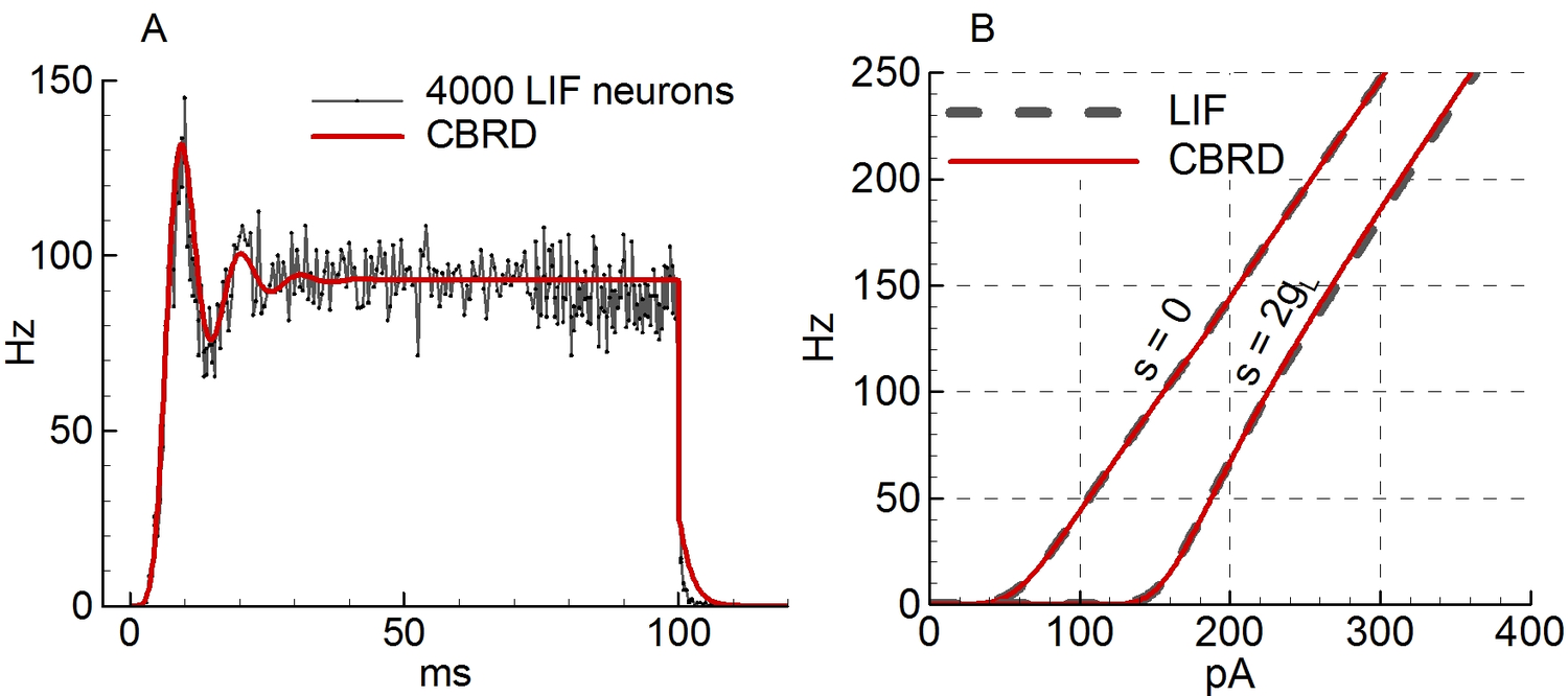
#1#2 #1#2 #1#2 #1#2 #1 + #1#2 #1#2#1 / #2 #1#2 #1#1 #1#2 #1#2 #1#1 #1#1 #1 #1 #1 #1 Conductance-based refractory density (CBRD) approach is an efficient approach that describes firing activity of a statistical ensemble of uncoupled Hodgkin-Huxley-like neurons each receiving individual gaussian noise and common time-varying deterministic input. However, the approach requires comparison with experiments and extension to the case of more realistic synaptic connectivity. Here we verify a CBRD model through comparison with experimental data and then generalize the model for the case of lognormal (LN) distribution of input weights within a population. We show that the model with equal weights efficiently reproduces post-spike time histogram and membrane voltage of experimental multiple-trial response of single neurons to step-wise current injection and reveals much more rapid reaction of firing-rate than voltage. Slow adaptive potassium channels strongly affect the shape of the responses. Next, we derive a computationally efficient CBRD model for a population with the LN input weight distribution and compare it to the original model with equal input weights. The analysis shows that the LN distribution does: (i) provide faster response; (ii) eliminate oscillations; (iii) lead to higher sensitivity to weak stimuli; (iv) increase the coefficient of variation of interspike intervals. In addition, a simplified, firing-rate type model is tested, showing better precision in the case of LN distribution of weights. More generally, the CBRD approach can be recommended for complex, biophysically detailed simulations of interacting neuronal populations, and the modified firing-rate type model for computationally reduced simulations. INTRODUCTION Known neuronal population models belong either to the type of very simplified models such as firing-rate (FR) or neural mass models or to those that are based on probability-density approach (PDA). FR-models are usually expressed by algebraic or ordinary differential equations and easy to analyze. However, they are not fully adequate for transient process simulations because of their basic assumption that neurons are always desynchronized. A probability density approach avoids this assumption, however this approach is commonly applied to simplified, one-variable neurons like linear and nonlinear integrate-and-fire, or spike-response model or so , , , , . This limitation has been overcome by a conductance-based refractory density approach (CBRD) that is applicable to regular-spiking, adaptive and fast-spiking neurons described in terms of Hodgkin-Huxley-like approximations . The CBRD approach has been proposed for an infinite set of such uncoupled neurons receiving a common input and an individual gaussian white noise-current. The model was later extended to the case of color noise . Such model is found to be quite efficient for simulation of coupled populations . The approach is worth being further developed and used in analysis of experimental data. In the present paper, the CBRD model is applied to experimental data revealing rapid population response to a weak input. Matching the model to experimental dataset validates the model, which then reveals the influence of neuronal parameters on the response. Further, the model is generalized for the case of lognormal distribution of the weights of the input received by different neurons of a population, which has many physiological implications . In addition, a simplified, firing-rate type model is tested to simulate a population with lognormal weights. METHODS For the purpose of clarifying the ideas of the CBRD-approach and its extension to the lognormal input weight distribution, we present in this section the models for simplified, integrate-and-fire neurons. The details of the model for adaptive Hogkin-Huxley like neurons can be found in or . _Leaky integrate-and-fire neuron with noise_ The LIF neuron is given by the equation C~{dV\over dt}=-(g_L+s(t)) (V-V_{rest}) + I(t) + \sigma ~\xi(t), where ξ(t) is a gaussian white noise characterized by its mean value, <ξ(t)> = 0, and auto-correlation <ξ(t)ξ(t′) > =C/gL δ(t − t′); σ is the noise amplitude. The neuron fires when the potential V crosses the threshold $\VT$. Immediately after the spike the potential V is reset to Vreset. The LIF neuron is characterized by the capacitance C and the leak conductance gL. The input is determined by two signals, the synaptic current I(t) that is measured at the voltage level equal to Vrest, and the total synaptic conductance s(t). The effective membrane time constant is τm = C/(gL + s(t)). We will refer to as a population an infinite number of eq.([e221])-based LIF neurons receiving a deterministic 2-d input (I(t),s(t)) and individual for each neuron noise. The population firing rate is defined as a sum of all spikes, nact, from neurons of the population over a short time window Δt, divided by the number of neurons, N. After taking the limits of N → ∞ and Δt → 0, the firing rate ν is obtained as \nu(t)= {\Delta t} ~(t;~t+\Delta t)}{N}. The steady-state firing rate is given by the solution from \nu^{SS}&=&\Biggl({g_L+s(t)} ~ -U)/\sigma_V \sqrt(2)}^{(\VT-U)/\sigma_V \sqrt(2)} \exp(u^2) (1+\erf(u)) ~du \Biggr)^{-1}, \\ U&=&V_{rest}+I/(g_L+S),\\ \sigma_V&=&{(g_L+s)} \\ where σV is the voltage dispersion; here U is the depolarization potential in the steady-state. _Conductance-based refractory density (CBRD) approach for a population of integrate-and-fire neurons_ As justified in , , the firing rate for a population of LIF neurons is well approximated by the system of equations for the refractory density $\rho(t,\ts)$ and the averaged across noise realizations membrane potential $U(t,\ts)$, where $\ts$ is the time elapsed since the last spike. Thereby, the CBRD method distinguishes neurons only according to their $\ts$-variable. In order words, the state of each neuron is parameterized by this phase variable. For the particular case of a LIF-neuron, its only state variable is V, whereas for more complex neuron models the other state variables, the gating variables of ionic channels, are also parameterized by $\ts$, which is the reduction to an only one phase variable description that rather precisely saves the information about neuronal states because of the same history of input for all neurons . Returning to LIF-neurons, the equations for $\rho(t,\ts)$ and $U(t,\ts)$ are as follows t +{\ts}&=&-\rho~ H(U), \\ C\Biggl(\derc Ut + \derc U{\ts} \Biggr) &=& -(g_L+s(t)) (U-V_{rest}) + I(t), where H is a hazard function which is defined below. The boundary conditions are \nu(t) \equiv \rho(t,0)=\int ^{\infty} \rho H d\ts and U(t, 0)=Vreset, where ν(t) is the population firing rate. When calculating the dynamics of a neuronal population, the integration of eq.([e242]) determines the distribution of not-noisy voltage U across $\ts$. The effect of crossing the threshold and the diffusion due to noise are evaluated by the H-function and affect the equation for ρ. The result of the integration of eq.([e241]) is the distribution of ρ across $\ts$ and the firing rate ν calculated from ([e2425]). The hazard function H is defined as the probability for a single neuron to generate a spike, if known actual neuron state variables. The hazard function H has been approximated in for the case of white noise and in for the case of color noise as a function of U(t) and s(t), and parameters σ, $\VT$ and the ratio of membrane to noise time constants k = τm/τNoise: H&(U)&= A+B,\\ A&=& %A_{0}&=& {\tau_m} e^{0.0061-1.12~T-0.257~T^2-0.072~T^3-0.0117~T^4} %\nonumber \\&\cdot& \biggl(1-(1+k)^{-0.71+0.0825(T+3)}\biggr),\nonumber \\ B&=&- ~ \biggl\lbrack {dT \over dt} \biggr \tilde F(T), ~~~\tilde F(T)= ~{\exp(-T^2) \over 1+\erf(T)},~~~ %\nonumber \\ T={~\sigma_V}, \nonumber where T is the membrane potential relative to the threshold, scaled by noise amplitude; A is the hazard for a neuron to cross the threshold because of noise, derived analytically in and approximated by exponential and polynomial for convenience; B is the hazard for a neuron to fire because of depolarization due to deterministic drive, i.e. the hazard due to drift in the voltage phase space. Note that the H-function is independent of the basic neuron model and does not contain any free parameters or functions for fitting to any particular case. In this aspect, the H-function can be useful not only as a component of a population model, but as well for analysis tasks such as evaluation of neuronal susceptibility , effects of noise etc. _Firing-rate model for integrate-and-fire neurons_ Conventional firing-rate type models often fail to describe well a population activity in transient states. A modified firing-rate model has been proposed in , which improves the transient solutions to step-like or complex-shape inputs . Below such model is given for the LIF-neuron population. The subthreshold voltage U(t) is calculated as C~{dU\over dt}=-(g_L+s(t)) (U-V_{rest}) + I(t), and the firing rate is calculated by the following formula \nu&=&\bigl[\nu^{SS} + \nu^{US} \bigr]_{+}, \\ \nu^{US}&=&{1 \over \sigma_V}{dU \over dt} \exp\Biggl( -{(\VT-U)^2 \over 2 \sigma_V^2} \Biggr), where the function [x]+ is defined as x for x > 0 and 0 otherwise. The term νSS is the steady-state solution ([e223]). The essence of the model modification consists in the term νUS, which evaluates the firing rate in response to fast excitation in assumption of a frozen gaussian distribution of neuronal membrane potentials crossing the threshold. RESULTS Validation of CBRD-model: comparison with analytical and Monte-Carlo solutions To validate the CBRD-model based on eqs.([e221]-[e223]) we compare it with Monte-Carlo (MC) simulation on a test problem of step-wise current stimulation. In MC simulations eq.([e221]) has been integrated 4000 times with different realizations of noise. The firing rate has been calculated from eq.([e2013]). As seen in Fig.[F-1]A, the CBRD and MC solutions are close; they converge with the increase of the number of neurons in MS simulations. For LIF neuron with white noise in steady-state, the analytical solution for the firing rate is known, it is given by eq.([e223]-[e225]). The CBRD-model matches to this solution with a high precision, as demonstrated by Fig.[F-1]B. Important, that the both solutions converge not only for variable input current but also for the input conductance. Comparison of CBRD-model with experimental data According to above introduced definition of a population, the neurons are independent from each other, thus, such population is equivalent to a number of noise realizations for a single neuron. Hence, statistics of the behavior of a neuron receiving both deterministic and stochastic inputs is governed by the same model as a single population. That is why, we compare the CBRD-model with experimental multiple registrations in a single neuron . A weak step-wise current was injected into the neuron. The statistics of spiking response is characterized by the post-stimulus spike-time histogram (PSTH) which corresponds to the firing rate for a population. The model has been taken from . In this model a basic single neuron had a few potassium ionic channels. The adaptation was taken into account in the forms of the M-current and the current of afterhyperpolarization (AHP-current) which effectively approximates the effects of potassium calcium-dependent currents. The spike trains in response to step-wise current injection reveals the similarity of the modeled and registered neuronal responses (compare Figure 1A,D in ) with Fig. [Fig1ABCD]A,C) and the effects of the adaptation. As to population response, the experimental PSTH (Figure 1E in ) is similar to the modeled firing rate (Fig. [Fig1ABCD]D). The response in the model is as fast as in the experiment, the timing of peaks, the amplitudes of the firing rate and the character of relaxation to the steady-state are similar. Also we find out similar rapid reaction to the change of the amplitude of noise (Fig. [Fig3B]). The most affective factors determining the shape of firing response are the level of background activity before the stimulus and the slow potassium channels (Fig. [Fig_SpontActivity_and_WhiteColorNoise]). As seen from comparison of Fig. [Fig_SpontActivity_and_WhiteColorNoise]C and D with Fig. [Fig_SpontActivity_and_WhiteColorNoise]B, the presence of spiking activity before the stimulus is critical for the rapidness of the response. The bigger the firing rate before stimulation the faster the response. This fact is consistent with the findings of the experimental study . Blockage of M- and AHP-currents crucially changes the later phases of the response, especially its steady-state, as seen from comparison of Fig. [Fig_SpontActivity_and_WhiteColorNoise]H with Fig. [Fig_SpontActivity_and_WhiteColorNoise]F. Regarding the time correlations of the noise, their effect is moderate (compare Fig. [Fig_SpontActivity_and_WhiteColorNoise]G with Fig. [Fig_SpontActivity_and_WhiteColorNoise]F). Derivation of CBRD-model for a population receiving lognormally distributed input Our goal is to generalize the CBRD-approach for a population of neurons receiving equal input I(t) and noise, that based on eqs.([e241]-[e243]), to the case of a population consisting of neurons receiving lognormally distributed deterministic inputs Ix(t). The distribution of the current Ix(t) scaled by its mean across the distribution I(t), x = Ix(t)/I(t), is as follows \psi(x)=/{(2~^2)}}\bigr)}{~ ~x} Let us consider neurons parameterized with x, i.e. those neurons that receive the deterministic input current Ix(t) as well as the input conductance s(t) and the noise σ ξ(t) introduced into eq.([e221]). The voltage averaged across realizations of the noise, to be denoted as Ux, is governed by eq.([e242]) written for Ux instead of U and Ix(t) instead of I(t). Such equation is linear in respect to Ix(t), thus the deflection of voltage $U_x(t,\ts)$ from the unperturbed state $U_{free}(\ts)$ (defined for zero input current I(t)=0) is also lognormally distributed in accordance to eq.([e3.1]), with its mean $U(t,\ts)-U_{free}(\ts)$ corresponding to the mean input current I(t). That is why, the voltage $U_x(t,\ts)$ can be found as U_x(t,\ts)=(U(t,\ts)-U_{free}(\ts))~x+U_{free}(\ts). It allows to reduce the consideration by avoiding direct solving of equations in partial derivatives for $U_x(t,\ts)$ on a semiinfinite space for x. Instead, the statistics for $U_x(t,\ts)$ is described by the single equation ([e242]), the distribution ([e3.1]) for x and the expression ([e3.3]). Now we derive equation for the neuronal density. The probability for a neuron with the voltage $U_x(t,\ts)$ to generate a spike is estimated by the hazard function H(Ux, dUx/dt). The distribution of neurons parameterized by x in the phase space $\ts$ is denoted as $\rho_x(t,\ts)$. Note that the distribution of $\rho_x(t,\ts)$ across x is not necessarily lognormal. Calculation of $\rho_x(t,\ts)$ require solving of a continuum of eqs.([e241]) for ρx instead of ρ with H(Ux, dUx/dt). The output firing rate is defined as \nu(t)=^{\infty} \rho_x(t,0) ~\psi(x)~dx The firing rate in the case of lognormal weight distribution of the deterministic input is calculated from eqs.([e241]-[e243], [e3.1]-[e3.2]). Because the extension of the numerical method of the calculations from that for the conventional method from is straightforward, the precision of the CBRD-model in this case is determined only by the parameters of integration. The values of the numerical parameters were chosen such that a residual error was less than 5%. The approximation of the distribution ([e3.1]) required 10-15 points of discretization; hence, the number of numerically integrated 1-d transport equations for ρx was equal to that number of points plus one (for U). Comparison of CBRD models with fixed and lognormally distributed input weights To reveal the difference between a population with equal weights and gaussian noise (P) and a population with lognormal distribution of weights (LNP) we considered again the task of step-wise current stimulation (Fig.[Fig_LNP_P_step]). The response of LNP is more rapid than both the voltage and the firing rate response of P, because of contribution of more sensitive neurons with strong weights from the tail of lognormal distribution. The LNP solution does not oscillate as the response of P, because of overlapping of contributions of the whole lognormal distribution. The steady-state firing rate is greater for LNP, because of nonlinear dependence of the firing rate on the input current for a single neuron (Fig. [F-1]B) and thus bigger contribution of the tail of lognormal distribution. The rapidness of the LNP response increases with the amplitude of stimulation (Fig. [Fig_3_ampl_step_and_sin]A). The sensitivity to weak stimulus is greater for LNP, again because of the contribution of the tail of lognormal distribution. In the steady-state, the lognormal distribution affects not only the firing rate but the interspike interval distribution also. According to the construction of the refractory density model, the distribution of interspike intervals is given by the source term in the eq.([e241]), i.e. ρ H, where ρ is the cumulative density $\rho(\ts)=^{\infty} \rho_x(\ts) ~\psi(x)~dx$. The coefficient of variation (CV) of interspike intervals for the whole population follows from the refractory density $\rho_x(\ts)$ and the hazard function H: CV=^{\infty} ^{\infty} \ts^2~\rho_x(\ts) H(U_x(\ts)) ~d\ts ~\psi(x)~dx %\rho_x(\ts) H(U_x(\ts)) ~\psi(x)~d\ts \\ / (E[\ts])^2 %\biggl( % ^{\infty} ^{\infty} \ts ~\rho_x(\ts) H(U_x(\ts)) ~\psi(x)~d\ts %\biggr)^2 -1 }, where \nonumber E[Z]= ^{\infty} ^{\infty} Z ~\rho_x(\ts) ~H(U_x(\ts)) ~\psi(x)~d\ts \big /~\nu % ^{\infty} ^{\infty} ~\rho_x(\ts) H(U_x(\ts)) ~\psi(x)~d\ts The dependence of the firing rate and CV on the input current I and the lognormal distribution dispersion σLN is plotted in Fig. [Fig_Iind_nu_CV]A. The CV strongly increases with σLN, which corresponds to the widening of the ISI distribution (ρH) shown in Fig. [Fig_Iind_nu_CV]B. Comparison of CBRD and firing-rate models We test the quality of solution obtained by the firing-rate model with lognormal distribution of weights (FR-LNP), based on eqs. ([e231]-[e234],[e223] and [e3.1]). As seen from Fig. [Fig_3_ampl_step_and_sin]A, the initial part of the response as well as the plateau of the steady-state are captured by the model. Good approximation of the rapid response at the initial stage is due to the term νUS in the eq.([e232]). The cumulative across the whole lognormal distribution action of this term provides the sharp profile. The most problematic is the phase of relaxation after the end of stimulation, the FR-LNP model shows too delayed relaxation. Better precision of the FR-LNP model is observed in the case of oscillatory input, as seen from Fig. [Fig_3_ampl_step_and_sin]B. DISCUSSION AND CONCLUSIONS The probability density approach and, in particular, the refractory density approach provides good approximation of firing rate calculation for a statistical ensemble of neurons in transient regimes of activity , , , , . Among these models, only the refractory density approach has been designed for complex, Hodgkin-Huxley like neurons , which was referred to as CBRD-model. Also important to note that the hazard-function derived for this model is more precise, does not contain any free forms or parameters for fitting and universal for different basic neuron models and input signal behavior, because it was strictly derived from the first-time passage problem for linearized voltage fluctuations about the time-variable mean near the threshold. These benefits of the model justifies the necessity of its further validation and development. In this paper some additional validations of the approach have been presented, namely its comparison to the alternative methods of firing rate calculation and experimental data. Further, the approach have been generalized to the case of lognormal distribution of “effective” synaptic weights, the weights of the input into neurons of a population. The CBRD model reveals rapidness and sensitivity of a population response to input changes. These properties are consistent with those found in exponential integrate-and-fire neurons and are physiological important for brain networks , . As pointed in , theoretical analysis identified three basic requirements for fast processing: use of neuronal populations for encoding, background activity, and fast onset dynamics of action potentials in neurons. All these requirements were satisfied in our simulations that have shown fast responses. In particular, the condition of the rapid initiation of action potentials , was fulfilled, because the CBRD-model uses threshold criterion for spike initiation, thus the initiation is instantaneous by the construction . The effect of background activity has been studied and found to be consistent with the experimental observations . Higher sensitivity is revealed in the case of lognormal distribution, which is explained by contribution of neurons from the tail of the distribution that are sparse but powerful. However this effect of the distribution is less pronounced than that for the interspike interval distribution. The coefficient of variation of intervals between spikes generated by the whole population as a measure of the interspike interval distribution strongly depends on the dispersion that characterizes the lognormal input weight distribution. Nevertheless, this coefficient does not relate directly to the dispersion of interspike intervals for a single neuron, which mechanism was studied in , etc. What is also important for simulations of interacting neuronal populations is mathematical complexity of a model and efficiency of its numerical solution. Regarding the CBRD approach, even in the case of realistic neurons and lognormal distribution its mathematical complexity is reduced to tens of one-dimensional transport equations, which are quite solvable numerically. Hence, computational efficiency of the method is comparable to that for population models with one-dimensional neurons and complex synaptic weight distributions, like in . Note, however, the difference between the proposed and the mentioned approach from . The synaptic weights were uncorrelated in time in that approach, whereas the proposed approach considers fixed distribution of weights for the deterministic input and temporally uncorrelated or colored individual noise. These assumptions seem to be more realistic. The above consideration allows one to conclude that the CBRD approach can be recommended as useful for cortical tissue simulations, because it provides significant gain in precision in comparison to conventional mean-field models, computational effectiveness in comparison with direct network simulations and the detail consideration of biophysical mechanisms in comparison with Fokker-Planck-based models; it also admits mathematical analysis of the system of equations. Regarding more simplified, firing-rate type population models, generally they fail to simulate correctly the transient regimes, however some modifications help to improve their quality , , . One of such models that was described in Methods was generalized for the case of lognormal distribution of input weights. Its comparison with the CBRD-model has revealed that the modified FR model provides more or less satisfactory approximation in the case of lognormal distribution. Thus, this model can also be recommended for simplified simulations. Acknowledgement This work was supported by the Russian Science Foundation (project 16-15-10201)