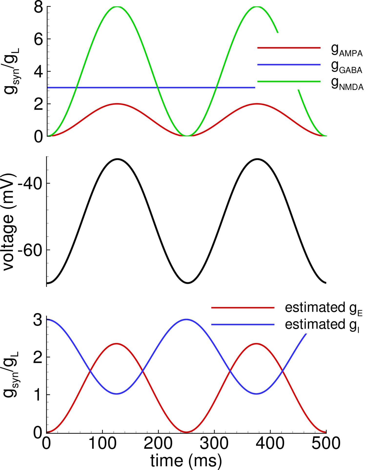
AUTHOREA
Log in Sign Up Browse Preprints
BROWSE LOG IN SIGN UP

Public Articles

Back to Browse
Sample Blog Post Math 381
Serge Ballif

Serge Ballif

January 12, 2016
Graphs and Digraphs A graph is a structure used in discrete math that is used to show the relationship between various objects. The objects form the vertices of the graph. Two vertices are connected by a line if they satisfy a certain relationship. We call these lines edges. By formalizing the way we connect the dots we are able to rigorously prove mathematical claims.
PHD Proposal
Jesse Greenslade

Jesse Greenslade

May 26, 2015
BACKGROUND
A quick introduction to version control with Git and GitHub
Alexey Voronov

Alexey Voronov

January 18, 2016
INTRODUCTION TO VERSION CONTROL Many scientists write code as part of their research. Just as experiments are logged in laboratory notebooks, it is important to document the code you use for analysis. However, a few key problems can arise when iteratively developing code that make it difficult to document and track which code version was used to create each result. First, you often need to experiment with new ideas, such as adding new features to a script or increasing the speed of a slow step, but you do not want to risk breaking the currently working code. One often utilized solution is to make a copy of the script before making new edits. However, this can quickly become a problem because it clutters your filesystem with uninformative filenames, e.g. analysis.sh, analysis_02.sh, analysis_03.sh, etc. It is difficult to remember the differences between the versions of the files, and more importantly which version you used to produce specific results, especially if you return to the code months later. Second, you will likely share your code with multiple lab mates or collaborators and they may have suggestions on how to improve it. If you email the code to multiple people, you will have to manually incorporate all the changes each of them sends. Fortunately, software engineers have already developed software to manage these issues: version control. A version control system (VCS) allows you to track the iterative changes you make to your code. Thus you can experiment with new ideas but always have the option to revert to a specific past version of the code you used to generate particular results. Furthermore, you can record messages as you save each successive version so that you (or anyone else) reviewing the development history of the code is able to understand the rationale for the given edits. Also, it facilitates collaboration. Using a VCS, your collaborators can make and save changes to the code, and you can automatically incorporate these changes to the main code base. The collaborative aspect is enhanced with the emergence of websites that host version controlled code. In this quick guide, we introduce you to one VCS, Git (git-scm.com), and one online hosting site, GitHub (github.com), both of which are currently popular among scientists and programmers in general. More importantly, we hope to convince you that although mastering a given VCS takes time, you can already achieve great benefits by getting started using a few simple commands. Furthermore, not only does using a VCS solve many common problems when writing code, it can also improve the scientific process. By tracking your code development with a VCS and hosting it online, you are performing science that is more transparent, reproducible, and open to collaboration . There is no reason this framework needs to be limited only to code; a VCS is well-suited for tracking any plain-text files: manuscripts, electronic lab notebooks, protocols, etc.
ProCS15: A DFT-based chemical shift predictor for backbone and C\(\beta\) atoms in pr...
Alexey Voronov

Alexey Voronov

January 18, 2016
ABSTRACT We present ProCS15: A program that computes the isotropic chemical shielding values of backbone and Cβ atoms given a protein structure in less than a second. ProCS15 is based on around 2.35 million OPBE/6-31G(d,p)//PM6 calculations on tripeptides and small structural models of hydrogen-bonding. The ProCS15-predicted chemical shielding values are compared to experimentally measured chemical shifts for Ubiquitin and the third IgG-binding domain of Protein G through linear regression and yield RMSD values below 2.2, 0.7, and 4.8 ppm for carbon, hydrogen, and nitrogen atoms respectively. These RMSD values are very similar to corresponding RMSD values computed using OPBE/6-31G(d,p) for the entire structure for each protein. The maximum RMSD values can be reduced by using NMR-derived structural ensembles of Ubiquitin. For example, for the largest ensemble the largest RMSD values are 1.7, 0.5, and 3.5 ppm for carbon, hydrogen, and nitrogen. The corresponding RMSD values predicted by several empirical chemical shift predictors range between 0.7 - 1.1, 0.2 - 0.4, and 1.8 - 2.8 ppm for carbon, hydrogen, and nitrogen atoms, respectively.
A quick introduction to version control with Git and GitHub
Alexey Voronov

Alexey Voronov

January 18, 2016
INTRODUCTION TO VERSION CONTROL Many scientists write code as part of their research. Just as experiments are logged in laboratory notebooks, it is important to document the code you use for analysis. However, a few key problems can arise when iteratively developing code that make it difficult to document and track which code version was used to create each result. First, you often need to experiment with new ideas, such as adding new features to a script or increasing the speed of a slow step, but you do not want to risk breaking the currently working code. One often utilized solution is to make a copy of the script before making new edits. However, this can quickly become a problem because it clutters your filesystem with uninformative filenames, e.g. analysis.sh, analysis_02.sh, analysis_03.sh, etc. It is difficult to remember the differences between the versions of the files, and more importantly which version you used to produce specific results, especially if you return to the code months later. Second, you will likely share your code with multiple lab mates or collaborators and they may have suggestions on how to improve it. If you email the code to multiple people, you will have to manually incorporate all the changes each of them sends. Fortunately, software engineers have already developed software to manage these issues: version control. A version control system (VCS) allows you to track the iterative changes you make to your code. Thus you can experiment with new ideas but always have the option to revert to a specific past version of the code you used to generate particular results. Furthermore, you can record messages as you save each successive version so that you (or anyone else) reviewing the development history of the code is able to understand the rationale for the given edits. Also, it facilitates collaboration. Using a VCS, your collaborators can make and save changes to the code, and you can automatically incorporate these changes to the main code base. The collaborative aspect is enhanced with the emergence of websites that host version controlled code. In this quick guide, we introduce you to one VCS, Git (git-scm.com), and one online hosting site, GitHub (github.com), both of which are currently popular among scientists and programmers in general. More importantly, we hope to convince you that although mastering a given VCS takes time, you can already achieve great benefits by getting started using a few simple commands. Furthermore, not only does using a VCS solve many common problems when writing code, it can also improve the scientific process. By tracking your code development with a VCS and hosting it online, you are performing science that is more transparent, reproducible, and open to collaboration . There is no reason this framework needs to be limited only to code; a VCS is well-suited for tracking any plain-text files: manuscripts, electronic lab notebooks, protocols, etc.
THE PREDICTION OF OUTCOMES RELATED TO THE USE OF NEW DRUGS IN THE REAL WORLD THROUGH...
Enzo Grossi

Enzo Grossi

January 17, 2016
THE PREDICTION OF OUTCOMES  RELATED TO THE USE OF NEW DRUGS IN THE REAL WORLD THROUGH ARTIFICIAL ADAPTIVE SYSTEMS.Enzo Grossi & Massimo Buscema Semeion Research CentreResearch Centre of Sciences of CommunicationVia Sersale 117, Rome, 00128, ItalyINTRODUCTIONIn this brief essay we will focus three main problems related to the use of new medications in the real world: 1) the prediction of drug response in individual patients; 2) the prediction of rare unwanted events after introduction of the new drug on the market; 3) the passage from preclinical phase to Phase I in human beings. The first problem is specifically felt by medical doctors who are asked to treat their patients as individuals rather than as statistics, but we have to note that, with the advent of extremely costly new drugs, also health authorities or private insurance organizations are looking for potent tools to personalize treatment plans. The second problem is typically sensed by drug agencies which sometimes are forced to withdraw marketing authorization as a bunch of deaths drug related creates rumors and disappointments at media level, while the third problem is specifically felt by Pharmaceutical Companies and Institutional Review Boards releasing the clearance for first in man trials.1.Prediction of drug response in individual patientMaking predictions for specific outcomes (diagnosis, risk assessment, prognosis) represents a fascinating aspect of medical science. Different statistical approaches have been proposed to define models to identify factors that are predictive for the outcome of interest. Studies have been performed to define the clinical and biological characteristics that could be helpful in predicting who will benefit from an antiobesity drug for example, but results have been limited (1).Traditional statistical approaches encounter problems when the data show big variability  and not easily normalized for inherent nonlinearity. More-advanced analysis techniques, such as dynamic mathematical models, can be useful because they are particularly suitable for solving nonlinear problems frequently associated with complex biological systems.Use of ANNs in biological systems has been proposed for different purposes, including studies on deoxyribonucleic acid sequencing (2) and protein structure (3).ANNs have been used in different clinical settings to predict the effectiveness of instrumental evaluation (echocardiography, brain single photon emission computed tomography, lung scintigram, prostate biopsy) in increasing diagnostic sensitivity and specificity and in laboratory medicine in general (4). Also, they have proven effective in identifying gastro-oesophageal refux patients on the sole basis of clinical data (5). But the most promising application of ANNs relates to prediction of possible clinical outcomes with specific therapy. ANNs have proven effective in detecting responsiveness to methadone treatments of drug addicts (6), to pharmacological treatment in Alzheimer disease (7), to clozapine in schizophrenic patients (8) and in various fields of psychiatric research (9). The use of ANNs for predictive modelling in obesity dates back to a decade ago, where it was proposed to model the waist-hip ratio from 13 other health parameters (10). Later, it has been proposed as a tool for body composition research (11). One of the main factors preventing a more efficient use of new pharmacological treatments  for chronic diseases like for example hypertension, cancer, Alzheimer disease or obesity is represented by the difficulty of predicting “a priori” the chance of response of the single patient to a specific drug.  A major methodological setback in drawing inferences and making predictions from data collected in the real world setting, such as observational studies, is that variability in the underlying biological substrates of the studied population and the quality and content of medical intervention influence outcomes. Because there is no reason to believe that these, like other health factors, work together in a linear manner, the traditional statistical methods, based on the generalized linear model, have limited value in predicting outcomes such as responsiveness to a particular drug. Most studies have shown that up to 50% of  patients treated with new molecules given in monotherapy or as an adjunct to standard  treatments may show an unsatisfactory response. As a matter of fact, when time comes for the physician to decide about type of treatment, there is very little evidence that can help her/him in drug treatment choice. Take for example obesity. Here only scanty data are available on predictive factors to the specific treatment, and attempts at developing models for predicting response to the drug by using traditional techniques of multiple regression have showed an unsatisfactory predictive capacity (i.e. inferior to 80% of total variance). (12, 13). A possible explanation could be that obesity is a so-called complex disease, where different factors interact with multiple interactions among variables, positive and negative feedback loops, and non-linear system dynamics. Another good example is Alzheimer Disease.Clinical trials have established the efficacy of cholinesterase inhibitor drugs (ChEI), such as tacrine,(14) donepezil, (15) and rivastigmine (16) based on improvement in cognitive aspects and in overall functioning using the Alzheimer’s Disease Scale—Cognitive subscale (ADAS-Cog)  and theClinician’s Interviewed Based Impression of Change (CIBIC)  , respectively. Although the mean score of treated patients in both scales was significantly higher than the placebo group, many subjects under active treatment showed little or no improvement (nonresponders).However it is not possible to estimate which patients are likely to respond to pharmacological therapy with ChEI. This prediction would be an important decision-making factor in improving the use of healthcare resources.A major methodological setback in drawing inferences and making predictions from data collected in the real world setting, such as observational studies, is that variability in the underlying biological substrates of the studied population and the quality and content of medical interventioninfluence outcomes. Because there is no reason, a priori, to believe that these, like other health factors, work together in a linear manner, the traditional statistical methods, based on the generalized linear model, have limited value in predicting outcomes such as responsiveness toa particular drug.A possible alternative approach to the solution of the problem is represented by the use of Neural Networks. Artificial Neural Networks (ANN) represent computerized algorithms resembling interactive processes of human brain. They allow to study very complex non-linear phenomena like biological systems. Like the brain, ANNs recognize patterns, manage data, and, most significantly, learn. These statistical-mathematical tools can determine the existence of a correlation between series of data and a particular outcome and when “trained” can predict output data once given the input. They work well in pattern recognition and discrimination tasks.Although ANNs have been applied to various areas of medical research, they have not been employed in obesity clinical pharmacology.ANN proved to be a useful method to discriminate between responders and non-responders, better than traditional statistical methods in our three experimental studies carried out with donepezil in Alzheimer disease and with sibutramine in obesity and with infliximab in Crohn disease.In a paper published in 2002 (7)  we have evaluated the accuracy of artificial neural networks compared with discriminant analysis in classifying positive and negative response to the cholinesterase inhibitor donepezil in a opportunistic  group of  61 old patients of both genders affected by Alzheimer’s disease (AD) patients in real world setting along three months follow-up.Accuracy in detecting subjects sensitive (responders) or not (nonresponders) to therapy was based on  the standard FDA criterion standard for evaluation of efficacy:  the scores of Alzheimer’s Disease Assessment Scale—Cognitive portion and Clinician’s Interview Based Impression of Change—plus scales. In this study ANNs were more effective in discriminating between responders and nonresponders than other advanced statistical methods, particularly linear discriminant analysis. The total accuracy in predicting the outcome was 92.59%.In a second study  we evaluated the use of artificial neural networks  in predicting response to infliximab treatment in patients with Crohn's disease(18).In this pilot study , different ANN models were applied to a data sheet with demographic and clinical data  from 76 patients with steroid resistant/dependant or fistulizing  CD treated with Infliximab to compare accuracy in classifying responder and non responder subjects with that of linear discriminant analysis.Eighty one  outpatients  with CD (31 men, 50 women;  mean age± standard deviation  39.9 ± 15  range: 12-81 ) partecipating to an Italian Multicentric Study (17) , were enrolled in the study.  All patients  were treated, between April 1999 and December 2003, with a dose of Infliximab 5 mg/kg of body weight  for  luminal refractory (CDAI > 220–400) (43 patients), fistulizing  CD (19 patients) or both of them (14 patients) .The final data  sheet consisted of 45 independent variables related to the anagraphic and anamnestic data (sex, age at diagnosis, age at infusion ,  smoking habit, previous Crohn’s related abdominal surgery [ileal or ileo-cecal resections] and concomitant treatments including immunomodulators and corticosteroids ) and to clinical aspects ( location of disease,  perianal disease, type of fistulas,  extraintestinal manifestations, clinical activity at the first infusion  [CDAI], indication for treatment). Smokers were defined as those smoking a minimum of 5 cigarettes per day for at least 6 months before their first dose of Infliximab.  Non smokers were defined as those who had never smoked before, those who had quit smoking at least 6 months before their first dose of Infliximab, or those who smoked fewer than 5 cigarettes per day. Concomitant immunosuppressive use was defined as initiation of methotrexate  before their first Infliximab infusion or initiation of 6-mercaptopurine (6-MP) or azathioprine more than 3 months before their first Infliximab infusion.Assessment of response was determined by clinical evaluation 12 weeks after the first infusion for all patients. Determination of response in patients with inflammatory CD was based on the Crohn’s Disease Activity Index (CDAI).  For clear - cut  estimate clinical response was evaluated as complete response or partial / no response.  Complete response was defined as  (a) clinical remission (CDAI < 150) in luminal refractory  disease and (b) temporary closure of all draining fistulas at consecutive visits in the case of enterocutaneous and perianal fistulas; entero-enteric  fistulas  were evaluated by  small bowel barium enema and vaginal vescical fistula  by lack  of drainage at consecutive visits . For patients with both indications  the outcome was evaluated independently for each indication.Two different experiments were planned following an identical  research protocol. The first one included all 45 independent variables including frequency and intensity Crohn disease symptoms, plus numerous other social and demographic characteristics, clinical features and history. In the second experiment the IS system coupled to the T&T system automatically selected the most relevant variables and therefore 22 variables were included in the model.Discriminant analysis was also performed on the same data sets to evaluate the predictive performance of this advanced statistical method by a statistician blinded to ANN results. Different models were assessed to optimise the predictive ability. In each experiment the sample was randomly divided into two sub-samples, one for the training phase and the other for the testing phase, with the same record distributions used for ANN validation.ANNs reached an overall accuracy rate of 88% while LDA performance was only of 72%.Finally in a third study we evaluated the performance of ANN in predicting response to Warfarin(17). A total of 377 patients were included in the analysis. The most frequent clinical indication for anticoagulation was atrial fibrillation (69%); other indications included heart valve prosthesis (10%) and pulmonary embolism (8%). The large majority of patients, 325, 86%) were on concurrent drug treatment: on average, they were taking 3 (IQR 1-4) medications potentially interacting with warfarin. The median weekly maintenance dose (WMD) of warfarin was 22.5 mg (IQR 16.3-28.8mg). Thirteen patients whose INR values were not within thetherapeutic range were erroneously included in the analysis: their median weekly maintenance dose was 21.4 mg (IQR 12.2-30.0 mg), the INR was higher than 3.0 (INR 3.7 and 4.3) in 2, and lower than 2.0 in 11 (median INR 1.5, IQR 1.5-1.7).Demographic, clinical and genetic data (CYP2C9 and VKORC1 polymorphisms) were used. The final prediction model was based on 23 variables selected by TWIST® system within a bipartite division of the data set (training and testing) protocol.TWIST system is based on a population of n ANNs, managed by an evolutionary system able to extracts from the global dataset the best training and testing sets and to evaluate the relevance of the different variables of the dataset in a sophisticated way, slecting the most relevant for the problem on study. The ANN algorithm reached high accuracy, with an average absolute error of 5.7 mg of the warfarin maintenance dose. In the subset of patients requiring ≤21 mg and 21-49 mg (45 and 51% of the cohort, respectively) the absolute error was 3.86 mg and 5.45 with a high percentage of subjects being correctly identified (71 and 73%, respectively). This performance is higher than those obtained in different studies carried out with traditional statistical techniques. In conclusion ANN appears to be a promising tool for vitamin K antagonist maintenance dose prediction.1.1 Selection of informative variables: how evolutionary algorithms workTo include only the most informative of the available variables we used a genetic algorithm, called the Genetic Doping Algorithm [19], which uses the principles of evolution to optimize the training and testing sets and to select the minimum number of variables capturing the maximum amount of available information in the data. Contrary to statistical linear models using indicator variables, TWIST does not require the omission of a reference category. This is due to the focus of the artificial neural network on prediction rather than estimation. If some of the indicator variables can completely account for the predictive ability of the others, those will be excluded by the algorithm during the selection process. The method is called the TWIST protocol and has been previously applied successfully in similar problems [20,21]. The advantages of the approach are the sub-setting of the data in two representative sets for training and testing, which is problematic in small datasets, and the use of a combination of criteria to determine the fit of the model. TWIST is comprised of two systems, the T&T for resampling of the data and the IS for feature selection, both using artificial neural networks (ANNs). The T&T system splits the data into training and testing sets in such a way that each subset is statistically representative of the full sample. This non-random selection of subsets is crucial when small samples are considered and the selection of non-characteristic and extreme subsets is likely. The IS system uses the training and testing subsets produced to identify a vector of 0s and 1s, describing the absence or presence of an indicator variable, that is able to optimize the categorization of the individuals in cases and controls compared to their observed status. For this, a population of vectors, with each vector a combination of the indicator variables, is allowed to “evolve” through a number of generations in order optimize the prediction of target variable, as a natural population evolves to optimize fitness under a specific set of environmental conditions. The vectors with the best predictive ability are overrepresented in the next generation while a smaller number of sub-optimal vectors are maintained to give rise to the following generation. Some instability, in the form of low predictive ability vectors, is introduced in the process to avoid the problem of finding a solution which is optimal under a narrow set of conditions, also known as a local optimum. This step ensures that the attributes do not include redundant information or noise variables that will decrease the accuracy of the map and increase both the computing time and the amount of examples necessary during learning. In addition, feature selection permits the easier interpretation of the graph of relationships between the variables. 2. Prediction of rare unwanted eventsDrug-induced injuries are a growing concern for health authorities. The world population is continuously growing older because of an increased life expectancy and is thus using more and more drugs, whether prescription or over-the-counter drugs.Therefore, chances of drug-induced injuries are rising. Over the years, a number of postmarketing labelling changes or drug withdrawals from the market due to postmarketing discoveries have occurred. Even the best planned and carefully designed clinical studies have limitations. To detect all potential adverse drug reactions, you need quite a large number of subjects exposed to the drug and the number of subjects participating in the clinical studies might not be large enough to detect especially rare adverse drug reactions.To minimise the risk of postmarketing discoveries such as unrecognised adverse drug reactions, certain risk factors, e.g. laboratory or ECG abnormalities, are subject of increased regulatory review.The most frequent cause of safety-related withdrawal of medications (e.g. bromfenac, troglitazone) from the market and for FDA non-approval is the drug-induced liver injury (DILI). Different degrees of liver enzyme elevations after drug intake can result in hepatotoxicity, which can be fatal due to the irreversible damage to the liver. Since animal models cannot always predict human toxicity, drug-induced hepatotoxicity is often detected after market approval. In the United States, DILI is contributing to more than 50% of acute liver failure cases (data from WM Lee and colleagues from the Acute Liver Failure Study Group).The second leading cause for withdrawing approved drugs from the market is QT interval prolongation, which can be measured during electrocardiogram (ECG). Some non-cardiovascular drugs (e.g. terfenadine) have the potential to delay cardiac repolarisation and to induce potentially fatal ventricular tachyarrhythmias such as Torsades de Pointes.Drug toxicity is also a common cause of acute or chronic kidney injury and can be minimised or prevented by vigilance and early treatment. NSAIDs, aminoglycosides, and calcineurin inhibitors are for example some drugs that are known to induce kidney dysfunction. Most events are reversible, with kidney function returning to normal when the drug is discontinued.Consequently, the pharmaceutical industry has a strong interest to identify drugs bearing the risk of causing adverse drug reactions as early as possible in order to improve the drug development programme. A patient developing a severe side effect to a particular medication can be considered an outlier. Suppose that you are deriving probabilities of future occurrences of severe side effects from the data collected in large clinical trials carried out  before the commercialization of your product. These trials provide healthy authorities that your product is effective and safe and so that its deserves a registration or marketing authorization.Now, say that you estimate that an event happens every 1,000 patients treated. You will need a lot more data than 1,000 patients to ascertain its frequency, say 3,000 patients. Now, what if the event happens once every 5,000 patients? The estimation of this probability requires some larger number, 15,000 or more. The smaller the probability, the more observations you need, and the greater the estimation error for a set number of observations. Therefore, to estimate a rare event you need a sample that is larger and larger in inverse proportion to the occurrence of the event. If small probability events carry large impacts ( in this example death), and (at the same time) these small probability events are more difficult to compute from past data itself, then our empirical knowledge about the potential contribution—or role—of rare events (probability × consequence) is inversely proportional to their impact. The future challenge in this particular setting will be to derive from the limited amount of information available in the pre registration  phase of drug development subtle, weak but true signals that something will go bad in the future after the marketing approval, when the new drug will be exposed in the real world to hundreds of thousand of subjects, a twofold increase in order of magnitude in comparison with pre-registration experience. These patients of the real world will be very different from patients encountered in the phase 3 clinical trial, generally speaking “clean patients” i.e. no concomitant disease, few concomitant treatments, age not beyond a certain value, good compliance, an so on. On the other hand in the post marketing phase the new drug will be exposed to “dirty patients” i.e subjects with substantial co-morbidity, many concomitant treatments, extreme age, poor compliance ( which mean also taking by mistake or intentionally excess of drug in the attempt to compensate for missed assumptions of the drug). Some artificial adaptive systems based on a new mathematics, could be able to learn from a large phase 3 study the hidden links among rare events and a particular profile of a patients even if no patients with such a particular profile actually exists in the data set.There are basically two possibilities: the first is to use an “associative memory” or autoassociative artificial neural network able to navigate in the hypersurface of a dataset in search of rare occurrence linked to a particular assembly of variables; the second is to use a pseudo-inverse function coupled with an evolutionary algorithms able to repopulate a specific probability density function distribution with virtual records enabling the search of rare events, not available in the original data set.2.1 Autoassociative artificial neural networks.The NR-NN is a new recurrent network provided with a new powerful algorithm (“Re-Entry” by the Semeion Research Centre), that can dynamically adapt its trajectory to answer according to the different questions, during the recall phase.This new artificial neural network, developing an associative memory, can identify the best possible connection between variables and can generate alternative data scenarios to follow the dynamic effects. During the training phase, the algorithm optimizes the weight of all the possible interconnections between variables in order to minimize the error. The training phase is followed by a rigorous validation protocol which foresees the correct reconstruction of variables that are randomly deleted by each record.During the querying phase of the database, the NR-NN can answer the following questions:• prototypical question (the characteristic prototype of a patient with a particular side effect or without a particular side effect),• virtual question (the prototypical profile of a patient having a side effect  with specific characteristics, even if no subject with these variables is actually present in the data set),These special dynamics of NR-NN allow us to distinguish 3 types of variables:• Discriminant variables: variables that are "switched on" only for a specific prototype;• Indifferent variables: variables that are "switched off" for both prototypes;• Metastable variables: variables that are "switched on" for both prototypes; in other words they act in opposite ways according to the context of the other variables. Metastable variables are specific of non-linear systems.The possibility to simulate rather than carrying out in reality a post marketing surveillance study in uncertain situations could help in optimizing decisions and save lives if the drug could cause severe side effects in rare patients.Actually there are  very few known computer aided simulators for clinical trials, for example the simulation method and the simulator proposed by Pharsight Corporation, Mountain View, California, USA. The basic features of the said known simulator is disclosed in “ Case Study in the use of Bayesian hierarchical modelling and simulation for design and analysis of a clinical trial, by William R. Gillespie, Bayesian CTS example at FDA/Industry workshop September 2003. The method on which the known simulator operates is a well known statistical algorithm known as “Montecarlo Algorithm”.This simulator however is not constructed in order to simulate the results or the trend of the results of a phase four  clinical trial. Thus the prediction cannot be seen as very reliable. The method furthermore is more oriented on better planning the trials relatively to the kind of individuals and the way the trials has to be carried out in order to have bigger chances of success.From theoretical point of view the use of Artificial Adaptive Systems should offer the possibility to infer results that are likely to be obtained in a advanced phase of marketing from the analysis of the data assembly related to the pre registrative phases. In other words the aim is to simulate and predict the results of post marketing surveillance from the data of phase 3, or better from an observational open study carried out in a large sample of the recipient population supposed to be exposed to the new drug after the commercialisation.  The only requirement is that this observational study would consists  in a assembly of a population not excessively “clean” but corresponding at least in part to the mix of variables encountered in the real world. The key point is to establish the “implicit function”  relating the input variables or independent variables, to the dependent variable ( specific outcome of a subject).It is interesting to note that at variance with classical statistics, which act on a particular data set with a vertical horizon, AAS tend to act with a horizontal approach. ( see figure 1).When the implicit function is established, for example with autoassociative neural networks, is possible to navigate on the hyper surface of the data set asking questions. For example one could ask which is the prototype of a subject having a specific negative outcome, and how this profile depend from the presence of the new drug. Let’s consider the problem of  drug-induced hepatotoxicity. During the Phase 3 clinical trials of a new drug the hepatic function has been closely monitored ad slight to moderate elevation of hepatic enzymes has been recorded in a small proportion of patients; for example 2% of the exposed population. Liver enzyme levels can range in a certain interval from zero to upper normal range till 10 times of the normal range in case  massive hepatic necrosis.Let’s take ALT: normal range is 1-20 units; a very high value is 400 units.In the trial 2% of patients showed elevation of ALT till 50 units; none of them had severe necrosis with very high ALT values.To adapt the collected data to neural network processing  scale the ALT values are scaled from 0 (equal to 1 ALT unit) to 1 ( equal to ALT 400 units).So a subject with ALT= 20 will be coded as 0.05; while a subject with ALT = 40 will be coded as 0.1.After the training phase with the auto-associative neural network, we ask the network which is the prototype of a patient with a very high ALT value, by setting the value of ALT in our scaled data set at 1.0 ( 400 units). During the query when ALT input is set on, the network will activate all its units in a dynamic, competitive and cooperative process at the same time..This external activation of ALT variable of the original dataset generates a process. Each step of this process is a state of a dynamical system. At each state, each variable will take a specific value, generated by the previous negotiation of that variable with all the others. The process will terminate when the system reaches its natural attractor. At this point, all the states of the process represent the prototype of the patients with strong elevation of ALT values. This prototype can be used to  monitor  patients candidate to receive the drug after commercialisation whose profile is close to the prototype.With the same approach we can generate prototype of patients having other severe reactions, as defined by dramatic changes of  specific  biomarkers.2.2 Pseudo-inverse function and evolutionary algorithmsA method for generating new records using an evolutionary algorithm (close to but different from a genetic algorithm) has been recently developed at Semeion Institute. This method, called Pseudo-Inverse Function (in short P-I Function), is able to generate new (virtual) data from a small set of observed data. P-I Function can be of aid when practical  constraints limit the number of cases collected during clinical trials, or in case of a population that shows some potentially interesting safety risk traits, but whose small size can seriously affect the reliability of estimates, or in case of secondary analysis on small samples. The applicative ground is given by research design with one or more dependent and a set of independent variables. The estimation of new cases takes place according to the maximization of a fitness function and outcomes a number as large as needed of ‘virtual’ cases, which reproduce the statistical traits of the original population. The algorithm used by P-I Function is known as Genetic Doping Algorithm (GenD), designed and implemented by Semeion Research Centre; among its features there is an innovative crossover procedure, which tends to select individuals with average fitness values, rather than those who show best values at each ‘generation’. A particularly thorough research design has been put on: (1) the observed sample is half-split to obtain a training and a testing set, which are analysed by means of a back propagation neural network; (2) testing is performed to find out how good the parameter estimates are; (3) a 10% sample is randomly extracted from the training set and used as a reduced training set; (4) on this narrow basis, GenD calculates the pseudo-inverse of the estimated parameter matrix; (5) ‘virtual’ data are tested against the testing data set (which has never been used for training). The algorithm has been validated on  a particularly difficult data set composed by only 44 respondents, randomly sampled from a broader data set taken from the General Social Survey 2002. The major result is that networks trained on the ‘virtual’ resample show a model fit as good as the one of the observed data, though ‘virtual’ and observed data differ on some features. It can be seen that GenD ‘refills’ the joint distribution of the independent variables, conditioned by the dependent one.This approach could be very interesting to expand the subset of patients who in the course of a clinical Phase 3 trial suffer for severe side effects. In the new virtual population thanks to the higher number of records it would be more appropriate to test statistical assumptions and derive predictive models.3.Prediction of drug toxicity dose-related in the passage from preclinical phase to Phase I in human beings.The recent disaster occurred in France where 5 healthy volunteers suffered from extremely severe Central nervous system  side effects following the administration of the highest dosage of a new chemical entity in the frame of dose-escalation Phase I clinical trial underlines the complexity to transfer data coming from animal studies to man choosing a dose range of medication with an acceptable risk of toxicity.Phase I studies are designed to test safety and tolerability of a drug, as well as how, and how fast, the chemical is processed by the human body. Most of these studies are carried out by specialized research contract companies; the subjects are usually healthy volunteers who receive modest financial compensation.Serious incidents in phase I studies are rare, but they can never be completely excluded because a drug's behavior in animals isn't always a good predictor of its effects in humans. The last publicly known similar incident occurred in 2006, when six men in the United Kingdom suffered severe organ dysfunction after receiving small doses of a monoclonal antibody named TGN1412.It is clear that differences in metabolic pathways in animal and human species, genetic predisposition, non linear pharmacokinetics of certain drugs, and other biological factor can interact  in a complex way giving rise to unexpected catastrophic event non commonly foreseeable with traditional mathematical approaches. These phenomena have to  do with chaos theory(22).A major breakthrough of the twentieth century, which has been facilitated by computer science, has been the recognition that simple rules not always lead to “ stable order,” but in many circumstances instead lead to an apparent disorder characterized by marked instability and unpredictable variation for reasons intrinsic to the rules themselves. The phenomenon of rules causing emerging disorder, counter-intuitive to many people, is the environment currently being explored as “self-organization,” “fractals,” i .e. (a fragmented geometric shape that can be split into parts, each of which is a reduced-size copy of the whole, a property called self-similarity), “non-linear dynamical systems” and “chaos.”Chaos theory, also called nonlinear systems theory, provides new insights into processes previously thought to be unpredictable and random. It also provides a new set of tools that can be used to analyze physiological and clinical data like for example unexpected reaction to pharmaceutical agents, electric signals coming from the heart or from the brain etc.Most of the reasoning in the section 2 of this essay applyies as well to this specific problem.in addition to autoassociative neural networksm evolutionary systems like those explained in section 1, when fed with adequate amount of information of different types, related to the pharmacological experiments performed in the preclinical development of a new drug can easily exploit a waste range of combinatorial occurrence and propose the safest protocol to be applied in healthy volunteers who for the first time will experiment the new compound. Evolutionary computation, offers practical advantages to the researcher facing difficult optimization problems. These advantages are multifold, including the simplicity of the approach, its robust response to changing circumstance, its flexibility, and many other facets. The evolutionary algorithm can be applied to problems  where heuristic solutions are not available or generally lead to unsatisfactory results.ConclusionsNew mathematical laws coupled by computer programming allow today to perform predictions which till few years ago were considered impossible. The prediction of response to a specific treatment in individual patients with supervised artificial neural networks has been documented and validated extensively in the literature. Less experience exists in predicting major unwanted effects of a new drugs after the commercialisation or predicting unexpected toxicity in Phase I clinical trials. In doing this task a close cooperation between regulatory agency scientific team and bio mathematicians experts in the use of new generations artificial adaptive system has to be strongly recommended..REFERENCES1) Padwal RS, Rucker D, Li SK, Curioni C, Lau DCW. Long-term pharmacotherapy for obesity and overweight. Cochrane database of Systematic Reviews 2003, Issue 4, Art. No.: CD004094. DOI:10.1002/14651858.CD004094.pub22) Parbhane RV, Tambe SS, Kulkarni BD. ANN modeling of DNA sequences: New strategies using DNA shape code. Comput Chem 2000;24:699–711.3) Jagla B, Schuchhardt J. Adaptive encoding neural networks for the recognition of human signal peptide cleavage site. Bioinformatics 2000;16:245–250.4) Tafeit E, Reibnegger G. Artificial neural networks in laboratory medicine and medical outcome prediction. Clin Chem Lab Med 1999;37:845–853.5) Pace F, Buscema M, Dominici P, Intraligi M, Baldi F, Cestari R, Passaretti S, Bianchi-Porro G, Grossi E. Artificial neural networks are able to recognize gastro-oesophageal reflux disease patients solely on the basis of clinical data. Eur J Gastroenterol Hepatol 2005; 6: 605-106) Massini G, Shabtay L. Use of a constraint satisfaction network model for the evaluation of the methadone treatments of drug addicts. Subst Use Misuse 1998;33:625–656.7) Mecocci P,Grossi E, Buscema M, Intraligi M, Savarè R, Rinaldi P, Cherubini A, Senin U. Use of Artificial Networks in Clinical Trials: A Pilot Study to predict Responsiveness to Donepezil in Alzheimer’s Disease. J Am Geriatr Soc 50:1857–1860, 2002.8) Lin CC, Wang YC, Chen JY, Liou YJ, Bai YM, Lai IC, Chen TT, Chiu HW, Li YC. Artificial neural network prediction of clozapine response with combined pharmacogenetic and clinical data. Comput Methods Programs Biomed. 2008; 91:91-9. 9) Politi E, Balduzzi C, Bussi R et al. Artificial neural network: A study in clinical psychopharmacology. Psychiatry Res 1999;87:203–215.10) Abdel-Aal RE, Mangoud AM. Modeling obesity using abductive networks. Comput Biomed Res. 1997;30: 451-71.11) Linder R, Mohamed EI, De Lorenzo A, Pöppl SJ. The capabilities of artificial neural networks in body composition research. Acta Diabetol. 2003;40 Suppl 1:S9-1412) Hansen D, Astrup A, Toubro S, Finer N, Kopelman P, Hilsted J, Rössner S, Saris W, Van Gaal L, James W, Goulder For The STORM Study Group M. Predictors of weight loss and maintenance during 2 years of treatment by sibutramine in obesity. Results from the European multi-centre STORM trial. Sibutramine Trial of Obesity Reduction and Maintenance.Int J Obes Relat Metab Disord. 2001;25:496-501.13) Hainer V, Kunesova M, Bellisle F, Hill M, Braunerova R, Wagenknecht M. Psychobehavioral and nutritional predictors of weight loss in obese women treated with sibutramine. Int J Obes 2005; 29: 208-16.14) Knopman D, Schneider L, Davis K et al. Long-term tacrine (Cognex) treatment.Effects on nursing home placement and mortality. Tacrine Study Group. Neurology 1996;47:166–177.15) Rogers SL, Farlow MR, Doody RS et al. A 24-week, double-blind, placebocontrolled trial of donepezil in patients with Alzheimer’s disease. Neurology 1998;50:136–145.16) Rösler M, Anand R, Cicin-Sain A et al. Efficacy and safety of rivastigmine in patients with Alzheimer’s disease: International randomised controlled trial. BMJ 1999;318:633–638.17) Grossi E, Podda GM, Pugliano M, Gabba S, Verri A, Carpani G, Buscema M, Casazza G, Cattaneo M. Prediction of optimal warfarin maintenance dose using advanced artificial neural networks. Pharmacogenomics. 2014 Jan;15(1):29-37. doi: 10.2217/pgs.13.212. PubMed PMID: 24329188.18) Kohn A, Grossi E, Mangiarotti R, Prantera C. Use of Artificial Neural Networks (ANN) in predictoring response to infliximab treatment in patients with Crohn’s disease. Dig Liver Dis 2005; 37 (suppl.1):S51.19) Buscema M (2004) Genetic doping algorithm (GenD): theory and applications. Expert Systems 21: 63–79.20) Buscema M, Grossi E, Intraligi M, Garbagna N, Andriulli A, Breda M (2005) An optimized experimental protocol based on neuro-evolutionary algorithms—Application to the classification of dyspeptic patients and to the prediction of the effectiveness of their treatment. Artificial Intelligence in Medicine 34: 279–305. PMID: 1602356421) Grossi E, Buscema M (2007) Introduction to artificial neural networks. European Journal of Gastroenterology & Hepatology 19: 1046–1054 doi: 10.1007/ s00535-009-0024-z PMID: 1930831022) Grossi E. Chaos theory.(2009) In: Encyclopedia of Medical Decision Making; Michael Kattan Ed.   pp. 129-132 SAGE Publications, Inc
Welcome to Authorea!
Alexey Voronov

Alexey Voronov

April 07, 2015
Hey, welcome. Double click anywhere on the text to start writing. In addition to simple text you can also add text formatted in BOLDFACE, _italic_, and yes, math too: E = mc²! Add images by drag’n’drop or click on the “Insert Figure” button.
Authenticating Route Transitions in an SPA: What to do About the Developer Console  
Alec Aivazis

Alec Aivazis

October 23, 2015
In a single page app, all of the decisions about what view/subview to render occurs on the client. This means that ideally the client would be able to authenticate the currently logged in user on transitions to sensitive pages and access its data without going back to the server. This means that special care needs to be made to protect our application from a malicious user interacting with the developer console present in all modern browsers. One possible security vulnerability is the escalation of a globally stored user user role. This would cause the hacker to view a part of the website that they were forbidden to.
Growth of 48 Built Environment Bacterial Isolates on Board the International Space St...
David Coil
Russell Neches

David Coil

and 6 more

April 02, 2015
ABSTRACT Background: While significant attention has been paid to the potential risk of pathogenic microbes aboard crewed spacecraft, much less has focused on the non-pathogenic microbes in these habitats. Preliminary work has demonstrated that the interior of the International Space Station (ISS) has a microbial community resembling those of built environments on earth. Here we report results of sending 48 bacterial strains, collected from built environments on earth, for a growth experiment on the ISS. This project was a component of Project MERCCURI (Microbial Ecology Research Combining Citizen and University Researchers on ISS). Results: Of the 48 strains sent to the ISS, 45 of them showed similar growth in space and on earth. The vast majority of species tested in this experiment have also been found in culture-independent surveys of the ISS. Only one bacterial strain that avoided contamination showed significantly different growth in space. _Bacillus safensis_ JPL-MERTA-8-2 grew 60% better in space than on earth. Conclusions: The majority of bacteria tested were not affected by conditions aboard the ISS in this experiment (e.g., microgravity, cosmic radiation). Further work on _Bacillus safensis_ could lead to interesting insights on why this bacteria grew so much better in space.
UZFor2015 - Timing Analysis Report
Tobias C Hinse

Tobias C Hinse

August 08, 2015
TIMING DATA The data has been taken from . All timing stamps are in BJD using the TDB time scale. No further transformations needed. A total of 42 timing measurements exist. However, Potter et al. have not included data points from Dai et al. (2010). See Potter et al. (2011) text for details. In this analysis I will consider the full set of timings as a start and as presented in Potter et al. (2011). LINEAR EPHEMERIS - FITTING A STRAIGHT LINE USING LINFIT In general I am using IDL for the timing analysis. The cycle or ephemeris numbers have been obtained from IDL> ROUND((BJDMIN-TZERO)/PERIOD) where BJDMIN are all 42 timing measurements, TZERO is an arbitrary timing measurement that defines the CYCLE=E=0 and PERIOD is the binary orbital period (0.087865425 days) and was taken from , Table 2. In this work I will use TZERO=BJD 2,450,021.779388. It is a bit different from the TZERO used in in order to introduce a bit variation and also because I think the center of mass of the data points is as chosen by me. As a first step I used IDL’s LINFIT code to fit a straight line with the MEASURE_ERROR keyword set to an array holding the timing measurements errors (Table 2, 3rd column, Potter et al. 2011). This way the square of deviations are weighted with 1/σ² where σ is the standard timing error for each timing measurement. This is standard procedure and was also used in Potter et al. (2011). The average or mean timing error for the 42 measurements is 6.0 seconds (the standard deviation is also 6.0 seconds) with 0.74 seconds as the smallest and 17 seconds as the largest error. Also I have rescaled the timing measurements by subtracting the first timing measurement from all the others. Rescaling introduces nothing spooky to the analysis and has the advantage to avoid dynamic range problems. This is in particular needed for a later analysis when using MPFIT. Using LINFIT the resulting reduced χ² value was 95.22 (χ² = 3808.82 with (42-2) degrees of freedom) with the ephemeris (or computed timings) given as T(E) = BJD~2450021.77890(6) + E \times 0.0878654291(1) The corresponding root-mean-square (RMS) scatter of the data around the best-fit line is 27.5 seconds and the corresponding standard deviation is 27.7 seconds. As expected they should both be similar. To measure scatter of data around any best-fit model, I will use the RMS quantity. The RMS scatter is  5 times the average timing error and could be indicative of a systematic process. As a test the CURVEFIT routine has been used in a similar manner. The resulting reduced chi2 was also 95.22 matching and confirming the result from the previous section. The /NODERIVATIVE keyword does not change anything and expressions for the partial derivative has been included. The RMS also agrees with the results obtained from LINFIT. However, the formal 1σ uncertainties in the best-fit parameters (TZERO and PERIOD) are one magnitude smaller compared to the equivalent values obtained from LINFIT. The data and the best-fit line (obtained from LINFIT) is shown in Fig. [linearfit] with the residuals plotted in Fig. [linearfit_res]. There is absolutely no difference when using the results from CURVEFIT. Linear ephemeris - conclusion After fitting a straight line and visually inspecting the residual plots I cannot see any convincing trend that should justify a quadratic ephemeris (linear + a quadratic term). What I see is a sinusoidal variation around the best-fit line. Relative to the linear line the first timing measurement arrives 20s earlier than expected. Then the trend goes down and increases again to 40s at E=0, then decreases again to a minimum to around 20s and increases again thereafter. There is no obvious quadratic trend from looking at the residuals in Fig. [linearfit_res]. QUADRATIC EPHEMERIS Although there is no obvious reason to include a quadratic term I will nevertheless consider a quadratic model. I will do this by again using IDL’s CURVEFIT procedure and the MPFIT package (also IDL) which is a more sophisticated fitting tool utilizing the Levenberg-Marquardt least-squares minimization algorithm developed by Marwardt. Quadratic ephemeris using CURVEFIT The results from CURVEFIT are surprising. The best-fit χ² value was 3718.89 yielding a reduced χ² of 95.36 with (42-3 DoF). The RMS scatter of the residuals around the quadratic model fit was 31 seconds. This means that the fit became worse compared to a linear ephemeris model. The resulting residual plot is shown in Fig. [quadfit_res]. The corresponding best-fit parameters along with formal uncertainties for a quadratic ephemeris are T(E) &=& T + P \times E + A \times E^2 \\ &=& 24550021.778895(6) + 0.0878654269(3) \times E + 4.3(5)\times 10^{-14} \times E^2 Quadratic ephemeris using MPFIT I have also used MPFIT to fit a quadratic ephemeris to the Potter et al. (2011) timing data. The resulting χ² is 3718.94 with (42-3) degrees of freedom yielding a reduced χ² of 95.36. This is identical to the results obtained with CURVEFIT and thus confirmed independently. This is really surprising. The RMS scatter of data around the quadratic ephemeris is around 31 seconds. I will not state the best-fit values for the three model parameters (and their uncertainties) as obtained from MPFIT. Quadratic ephemeris - conclusion Based on the above result I cannot see that the residuals relative to a linear ephemeris allow the inclusion of a secular term accounting for a quadratic ephemeris. The χ² increases with an extra parameter which is not what is expected. I will continue now and fit a 1- and 2-companion model. LINEAR + 1-COMPANION LTT MODEL USING MPFIT We have considered a linear + 1-LTT model (excluding secular changes as described in a quadratic ephemeris). We have again used MPFIT for this task. The model is taken from Irwin (19??). We considered 10⁷ initial guesses. The initial guess for the reference epoch and binary period were taken from the best-fit obtained from a linear ephemeris model. Inital guesses for the semi-amplitude of the light-time orbit were taken from an estimate of the amplitude as shown in Fig. 2. Initial guesses for the eccentricity covered the interval [0,0.9995]. Initial guess for the argument of pericenter covered the interval [0,360] degrees. Initial guess for the orbital period was also estimated from Fig. 2. Initial guess for the time of pericenter passage were obtained from T0 and the orbital period of the light-time orbit. Initial guesses were drawn at random. The methodology follows the same techniques as described in Hinse et al. (2012). Best-fit parameters were obtained from the best-fit solution covariance matrix as returned by MPFIT. Parameters errors should be considered as formal. The best-fit had a χ² = 185.2 with (42-7) degrees of freedom resulting in a reduced χν² = 5.3. The corresponding RMS scatter of data points around the best-fit is 15.7 seconds. The best-fit parameters are listed in Table [BestFitParamsLinPlus1LTT] and shown in Fig. [BestFitModel_LinPlus1LTT]. Recalling the average timing error (of 42 timing measurements) to be 6 seconds, that means that the RMS residuals are on a 2.6σ level. --------------- ------------------------------ T₀ (BJD) 2, 450, 021.77924 ± 3 × 10−5 P₀ (days) 0.0878654289 ± 2 × 10−10 asinI (AU) 0.00043 ± 2 × 10−5 e 0.65 ± 0.03 ω (radians) 6.89 ± 0.04 Tp (BJD) 2, 408, 616.0 ± 50 P (days) 6020 ± 35 RMS (seconds) 15.7 --------------- ------------------------------ : Best-fit parameters for a linear + 1-LTT model (full data set: 42 data points) COMPILING A NEW DATASET At the present stage some inconsistencies were discovered in the reported timing uncertainties as listed in Table 1 in Potter et al. (2011). For example the timing uncertainty reported by is 0.000023 days, while Potter et al. (2011) reports 0.00003 and 0.00004 days. Furthermore, after scrutinizing the literature we found that several timing measurements were omitted in Potter et al. (2011). We tested for the possibility that Potter et al. (2011) adopts timing uncertainties from the spread of data around a best-fit linear regression. However, that seems not the case: As a test, we used the five timing measurements from as listed in Table 1 in Potter et al. (2011). We fitted a linear straight line using CURVEFIT as implemented in IDL and found a scatter of 0.00004 to 0.00005 days depending on the metric used to measure scatter around the best-fit. The quoted uncertainties in Potter et al. (2011) are smaller by at least a factor of two. We conclude that Potter et al. (2011) must be in error when quoting timing uncertainties in their Table 1. Similar mistakes when quoting timing uncertainties apply to data listed in . Furthermore, after scrutinizing the literature for timing measurements of UZ For we found several timing measurements that were omitted in Potter et al. (2011). For example six eclipse timings were reported by with a uniform uncertainty of 0.00006 days. However, Potter et al. (2011) only reports three of the six timings. Furthermore, a total of five new timings were reported by , but only one were listed in Potter et al. (2011). We can not come up with a good explanation why those extra timing measurements should be omitted or discarded. All of the new data points have been presented in the original works alongside with data points used in the analysis of Potter et al. (2011). In this research we make use of all timing measurements that have been obtained with reasonable accuracy. We have therefore recompiled all available timing measurements from the literature. We list them in Table [NewTimingData]. The original HJD(UTC) time stamps from the literature were converted to the BJD(TDB) system using the on-line time utilities[1] . Not all sources of timing measurements provide explicit information of the the time standard used. In that case we assume that HJD time stamps are valid in the UTC standard. This assumption is to some extend justified since the first timing measurement was taken in august 1983. At that time the UTC time standard for astronomical observations was widespread. All new measurements presented in were taken directly from their Table 1. Some remarks are at place. By finding additional timing measurements (otherwise omitted in Potter et al. 2011) in the literature we decided to follow a different approach to estimate timing uncertainties. For measurements that were taken over a short time period one can determine a best-fit line and estimate timing uncertainties from the data scatter. The underlying assumption in this method is that no significant astrophysical signal (interaction between binary components or additional bodies) is contained in the timing measurements over a few consecutive observing nights. Therefore, the scatter around a linear ephemeris should be a reasonable measure of how well timings were measured. In other words, only a first-order effect due to a linear ephemeris is observed. Higher-order eclipse timing variation effects are negligible for data sets obtained during a few consecutive nights. The advantage is that for a given data set the same telescope/instrument were used as well as weather conditions were likely not to have changed much from night to night. Furthermore, most likely the same technique was applied to infer the individual time stamps of a given data set. In Table [NewTimingData] we list the original quoted uncertainties presented in the literature as σlit. We also list the uncertainty obtained from the scatter of the data around a best-fit linear regression line. The corresponding reduced χ² statistic for each fit is also tabulated in the third column. From the reduced χ² for each data set one can scale the corresponding uncertainties such that χν² = 1 is enforced . This step is only permitted if a high confidence in the applied model is justified. We think that this is the case when time stamps have been obtained over a short time interval. However, ultimately the timing uncertainty depends on the sampling of the eclipse event at a sufficiently high signal-to-noise ratio. The data set was split in two since those time stamps were obtained from two observing runs each lasting for a few days. Furthermore, we have calculated three data scatter metrics around the best-fit line: a) the root-mean-square, b) the standard deviation and c) the standard deviation as given by and defined as \sigma^2 = {N-2} ^{N}(y_{i} - a - bx_{i})^2 where N is the number of data points, a, b the two parameters for a linear line and (xi, yi) is a given timing measurement at a given epoch. We have tested the dependence of scatter on the weight used and found no difference in the scatter metrics when applying a weight of one for all measurements. Finally some additional details need to be mentioned. We only inferred new timing uncertainties for data sets with more than two measurements. For a given data set we used the published ephemeris (orbital period) to calculate the eclipse epochs. For the time stamps presented in no ephemeris was stated. We therefore, used their eclipse cycles for the independent variable to calculate a best-fit line. The reference epoch in each fit was placed to be in or near the middle of the data set. Two data points were discarded in the present analysis. We removed one time stamp from due to a too high timing uncertainty. Another time stamp was removed from the new data presented in Potter et al. (2011), namely the time stamp BJD(TDB) 2,454,857.36480850. This eclipse is duplicated as it was observed also with the much larger SALT/BVIT instrument resulting in a lower timing error. We therefore use only the SALT/BVIT measurement in the present analysis which makes use of a total of 54 timing stamps. The average or mean timing error for the 54 measurements is 5.7 seconds (the standard deviation is 6.5 seconds) with 0.33 seconds as the smallest and 26.5 seconds as the largest error. Also we have rescaled the timing measurements by subtracting the first time stamp from all the others. Rescaling introduces nothing spooky to the analysis and has the advantage to avoid dynamic range problems when carrying out the process of least-squares minimization. The total baseline of the data set spans  27 years. BJD(TDB) σlit χν² σlit, scaled σRMS STD Eq. [BevEq6p15] Remarks ---------------- ----------- ------- -------------- ----------- ----------- ----------------- ------------------------------------------------- 2455506.427034 0.0000100 – – – – – HIPPO/1.9m, 2455478.485831 0.0000100 – – – – – HIPPO/1.9m, 2455450.544621 0.0000100 – – – – – HIPPO/1.9m, 2454857.364805 0.0000086 – – – – – SALT/BVIT, 2454417.334722 0.0000086 – – – – – SALT/SALTICAM, 2453408.288086 0.0000086 0.198 3.83E-6 0.0000070 0.0000070 0.0000100 UCTPOL/1.9m, 2453407.321574 0.0000100 0.198 4.45E-6 0.0000070 0.0000070 0.0000100 UCTPOL/1.9m, 2453405.300663 0.0000350 0.198 1.56E-5 0.0000070 0.0000070 0.0000100 UCTPOL/1.9m, 2453404.334042 0.0000600 – – – – – SWIFT, 2452494.839196 0.0000870 – – – – – XMM OM, 2452494.575626 0.0000350 – – – – – UCTPOL/1.9m, 2452493.609058 0.0000700 – – – – – UCTPOL/1.9m, 2451821.702394 0.0000100 – – – – – WHT/S-Cam, 2451528.495434 0.0000200 0.134 7.32E-6 0.0000040 0.0000050 0.0000070 WHT/S-Cam, 2451528.407579 0.0000200 0.134 7.32E-6 0.0000040 0.0000050 0.0000070 WHT/S-Cam, 2451522.432730 0.0000200 0.134 7.32E-6 0.0000040 0.0000050 0.0000070 WHT/S-Cam, 2450021.779400 0.0000600 2.237 8.97E-5 0.0000500 0.0000600 0.0000900 CTIO 1m/photometer, set II, 2450021.691660 0.0000600 2.237 8.97E-5 0.0000500 0.0000600 0.0000900 CTIO 1m/photometer, set II, 2450018.704120 0.0000600 2.237 8.97E-5 0.0000500 0.0000600 0.0000900 CTIO 1m/photometer, set II, 2449755.634995 0.0000600 0.427 3.92E-5 0.0000200 0.0000300 0.0000300 CTIO 1m/photometer, set I, 2449755.547165 0.0000600 0.427 3.92E-5 0.0000200 0.0000300 0.0000300 CTIO 1m/photometer, set I, 2449753.614046 0.0000600 0.427 3.92E-5 0.0000200 0.0000300 0.0000300 CTIO 1m/photometer, set I, 2449752.647586 0.0000600 0.427 3.92E-5 0.0000200 0.0000300 0.0000300 CTIO 1m/photometer, set I, 2449733.405017 0.0000400 – – – – – EUVE, 2449310.332595 0.0000230 – – – – – EUVE, 2449276.680076 0.0000230 – – – – – EUVE, 2448784.721419 0.0000300 – – – – – HST, 2448483.606635 0.0000200 4.413 4.20E-5 0.0000300 0.0000400 0.0000400 ROSAT, 2448483.430915 0.0000200 4.413 4.20E-5 0.0000300 0.0000400 0.0000400 ROSAT, 2448483.343045 0.0000200 4.413 4.20E-5 0.0000300 0.0000400 0.0000400 ROSAT, 2448482.903785 0.0000200 4.413 4.20E-5 0.0000300 0.0000400 0.0000400 ROSAT, 2448482.727955 0.0000200 4.413 4.20E-5 0.0000300 0.0000400 0.0000400 ROSAT, 2447829.184858 0.0000600 0.120 2.08E-5 0.0000170 0.0000190 0.0000200 AAT, 2447829.096998 0.0000600 0.120 2.08E-5 0.0000170 0.0000190 0.0000200 AAT, 2447829.009088 0.0000600 0.120 2.08E-5 0.0000170 0.0000190 0.0000200 AAT, 2447828.130518 0.0000600 0.120 2.08E-5 0.0000170 0.0000190 0.0000200 AAT, 2447828.042638 0.0000600 0.120 2.08E-5 0.0000170 0.0000190 0.0000200 AAT, 2447827.954778 0.0000600 0.120 2.08E-5 0.0000170 0.0000190 0.0000200 AAT, 2447437.920514 0.0000300 – – – – – 2.3m Steward obs., 2447128.809635 0.0009000 0.059 2.18E-4 0.0002000 0.0002000 0.0002000 2.3m Steward obs., 2447128.722035 0.0009000 0.059 2.18E-4 0.0002000 0.0002000 0.0002000 2.3m Steward obs., 2447127.843835 0.0009000 0.059 2.18E-4 0.0002000 0.0002000 0.0002000 2.3m Steward obs., 2447127.755635 0.0009000 0.059 2.18E-4 0.0002000 0.0002000 0.0002000 2.3m Steward obs., 2447145.064339 0.0000600 1.046 6.14E-5 0.0002000 0.0002000 0.0003000 AAT, 2447127.227739 0.0003000 1.046 3.07E-4 0.0002000 0.0002000 0.0003000 AAT, 2447127.139439 0.0003000 1.046 3.07E-4 0.0002000 0.0002000 0.0003000 AAT, 2447097.792555 0.0002500 0.069 6.58E-5 0.0000600 0.0000500 0.0000700 ESO/MPI 2.2m, 2447094.717355 0.0002300 0.069 6.05E-5 0.0000600 0.0000500 0.0000700 ESO/MPI 2.2m, 2447091.554235 0.0002300 0.069 6.05E-5 0.0000600 0.0000500 0.0000700 ESO/MPI 2.2m, 2447090.587785 0.0001200 0.069 3.16E-5 0.0000600 0.0000500 0.0000700 ESO/MPI 2.2m, 2447089.709005 0.0003000 0.069 7.89E-5 0.0000600 0.0000500 0.0000700 ESO/MPI 2.2m, 2447088.742545 0.0003000 0.069 7.89E-5 0.0000600 0.0000500 0.0000700 ESO/MPI 2.2m, 2446446.973823 0.0001600 – – – – – EXOSAT, 2445567.177636 0.0001600 – – – – – EXOSAT, : 54 mid-eclipse times of the main accretion spot of UZ For. BJD(TDB) are barycentric Julian date time stamps in the TDB time system. All figures are in units of days. The time span of various data sets are as follows: ESO/MPI 2.2m: 9.0 days; AAT (Ferrario 1989): 18 days; 2.3m Steward obs. (Berriman 1988): 1 day; AAT (Bailey & Cropper 1991): 1 day; ROSAT (Ramsay 1994): 0.9 days; CTIO (Imamura et al. 1998, all data): 270 days; CTIO (Imamura et al. 1998, set I): 3 days; CTIO (Imamura et al. 1998, set II): 3 days; WHT/S-Cam (Perryman et al. 2001): 6 days; UCTPOL/1.9m (Potter et al. 2011): 3 days. The data from HIPPO/1.9m (Potter et al. 2011) were taken as presented in their paper due to a too long time span of any 3-point data set of which the shortest is around 50 days. A COMMENT ON THE USE OF F-TEST In this work we are not using the F-test as a statistical tool to perform model selection. The F-test is based on the assumption that uncertainties are Gaussian. This assumption might be violated if the data is affected by time-correlated red noise due to atmospheric effects and/or additional astrophysical effects that influence the shape of the eclipse profile. There exist no studies in the literature that has addressed this question and therefore we judge that the outcome of an F-test is unreliable. NEW DATASET WITH SCALED ERRORS: LINEAR EPHEMERIS USING MPFIT In the following we will consider the newly compiled data set with timing uncertainties obtained from rescaling the published uncertainties in order to ensure χ² = 1 over short time intervals. We have determined the following linear ephemeris using MPFIT. We followed the monte-carlo approach and determined a best-fit model by generating 10 million random initial guesses. We used best-fit parameters from LINFIT to obtain a first estimate of the initial epoch and period. Then initial guesses were drawn from a Gaussian distribution centered at the LINFIT values with standard deviation given by five times the formal LINFIT uncertainties. The linear ephemeris is shown in Fig. [Linearfit_NEW]. The resulting reduced χ² value was 162.5 (χ² = 8448.6 with (54-2) degrees of freedom) with the ephemeris (or computed timings) given as T(E) = BJD_{TDB}~2,450,018.703604(3) + E \times 0.08786542817(9) Residuals are shown in Fig. [Linfit_NEW_Res] and displays a systematic variation. The corresponding RMS scatter of the data around the best-fit line is 28.9 seconds. The scatter is  5 times the average timing error and could be indicative of a systematic process of astrophysical origin. NEW DATASET WITH SCALED ERRORS: QUADRATIC EPHEMERIS USING MPFIT We have also considered a quadratic model to the new data set. However, and judged by eye from Fig. [Linfit_NEW_Res], there is no obvious upward or downward parabolic trend in the data. Nevertheless we added a quadratic term and generated 10 million initial guesses to find a best-fit model. The resulting reduced χ² value increased to 165.7 with 54-3 degrees of freedom. We therefore, decide to not consider a quadratic ephemeris in our further analysis. NEW DATASET WITH SCALED ERRORS: LINEAR EPHEMERIS + 1-LTT MODEL USING MPFIT Using scaled uncertainties we have considered a linear + 1-LTT model. We have again used MPFIT. The model is taken from Irwin (19??) and described in Hinse et al. (2012). We considered 10⁷ initial guesses. The initial guess for the reference epoch and binary period were taken from the best-fit obtained from a linear ephemeris model. Inital guesses for the semi-amplitude of the light-time orbit were taken from an estimate of the amplitude as shown in Fig. 2. Initial guesses for the eccentricity covered the interval [0,1]. Initial guess for the argument of pericentre covered the interval [0,360] degrees. Initial guess for the orbital period was also estimated from Fig. [Linfit_NEW_Res]. Initial guess for the time of pericentre passage were obtained from T0 and the orbital period of the light-time orbit. Initial guesses were drawn at random. The methodology follows the same techniques as described in Hinse et al. (2012). Best-fit parameters were obtained from the best-fit solution covariance matrix as returned by MPFIT. Parameters errors should be considered as formal [OFF-THE-RECORD: FINAL ERRORS WILL USE BOOTSTRAP TECHNIQUE]. The best-fit had a χ² = 717.6 with 47 degrees of freedom resulting in a reduced χν² = 15.3. The corresponding RMS scatter of data points around the best-fit is 20.0 seconds. The best-fit parameters are listed in Table [BestFitParamsLinPlus1LTT_New_AllData] and shown in Fig. [BestFitModel_LinPlus1LTT_New_AllData]. Recalling the average timing error to be 6 seconds, that means that the RMS residuals are on a 3.3σ level indicating a significant signal of some origin. However, upon close inspection of Fig. [BestFitModel_LinPlus1LTT_New_AllData] the origin of the large scatter is mainly due to data obtained by , , and a single point from located between cycle number -27,000 and -35,000. In the following we investigate the effect of the resulting model when removing those data points. --------------- ------------------------------ T₀ (BJD) 2, 450, 021.77919 ± 3 × 10−5 P₀ (days) 0.0878654283 ± 1 × 10−10 asinI (AU) 0.00048 ± 3 × 10−5 e 0.76 ± 0.03 ω (radians) 3.84 ± 0.04 Tp (BJD) 2, 461, 743.0 ± 53 P (days) 5964 ± 25 RMS (seconds) 20.0 χ² 717.6 red. χ² 15.3 --------------- ------------------------------ : Best-fit parameters for a linear + 1-LTT model (full data set: 54 data points with scaled error bars). NEW DATASET WITH SCALED ERRORS (WITH REMOVED DATA I): LINEAR EPHEMERIS + 1-LTT MODEL USING MPFIT To start we have removed a total of eight points: three points from , four points from and a single point from . The average deviation of those points from our best-fit model (Fig. [BestFitModel_LinPlus1LTT_New_AllData] and Table [BestFitParamsLinPlus1LTT_New_AllData]) was around 35 seconds. The minimum timing uncertainty is 0.33 seconds. The maximum timing uncertainty is 13.8 seconds. The mean of the timing uncertainty is 3.7 seconds. This data set is very similar to the data set investigated by Potter et al. (2011). Our new model now had a χ² = 467.1 and a reduced χ² = 12 with 39 DoF resulting in a RMS scatter of 13 seconds. We show the resulting best-fit parameters in Fig. [BestFitModel_LinPlus1LTT_RedDataSet1] and Table [BestFitParamsLinPlus1LTT_RedDataSet1]. As a result we first note that the removal of eight data points did not change significantly the model. This points towards that those discarded points do not contribute significantly to constrain the model during the fitting process. Further we note that our model is significantly different from the first elliptical term model presented in Potter et al. (2011). The most striking difference is dominantly seen in the eccentricity parameter. While they found a near-circular model we find a highly eccentric solution. Next we continue our analysis by removing an additional six data points. --------------- ------------------------------ T₀ (BJD) 2, 450, 021.69149 ± 4 × 10−5 P₀ (days) 0.0878654287 ± 1 × 10−10 asinI (AU) 0.00047 ± 3 × 10−5 e 0.73 ± 0.04 ω (radians) 0.74 ± 0.03 Tp (BJD) 2455832.0 ± 28 P (days) 6012 ± 23 RMS (seconds) 13.0 χ² 467.1 red. χ² 12.0 --------------- ------------------------------ : Best-fit parameters for a linear + 1-LTT model. A total of eight data points from , and were removed. NEW DATASET WITH SCALED ERRORS (WITH REMOVED DATA II): LINEAR EPHEMERIS + 1-LTT MODEL USING MPFIT In this section we investigate the effects by removing a total of 14 data points. Six from , three from , four points from and a single point from . The minimum timing uncertainty is 0.33 seconds. The maximum uncertainty is 13.8 seconds and the mean is 3.5 seconds. The resulting best-fit model is shown in Fig. [BestFitModel_LinPlus1LTT_RedDataSet2] with best-fit parameters listed in Table [BestFitParamsLinPlus1LTT_RedDataSet2]. We note that the resulting best-fit model has not changed significantly. Also the RMS scatter is comparable with the mean timing uncertainty. From this we can conclude that the timing errors should be scaled with $$ if the model is the correct description of the signal. --------------- ------------------------------ T₀ (BJD) 2, 450, 021.69150 ± 3 × 10−5 P₀ (days) 0.0878654279 ± 1 × 10−10 asinI (AU) 0.00049 ± 3 × 10−5 e 0.79 ± 0.03 ω (radians) 6.91 ± 0.03 Tp (BJD) 2467502 ± 57 P (days) 5901 ± 20 RMS (seconds) 4.4 χ² 161.0 red. χ² 4.9 --------------- ------------------------------ : Best-fit parameters for a linear + 1-LTT model. A total of 14 data points from , , and were removed. NEW DATASET WITH SCALED ERRORS (WITH REMOVED DATA III): LINEAR EPHEMERIS + 1-LTT MODEL USING MPFIT Finally, we have also discarded the two first timing measurements from . The mean timing uncertainty is 3 seconds. Again we found a best-fit model as shown in Fig. [BestFitModel_LinPlus1LTT_RedDataSet3] with best-fit parameters listed in Table [BestFitParamsLinPlus1LTT_RedDataSet3]. Also in this case the model did not change much compared to previous investigations. This points towards that the data taken at earlier epochs (discarded) does not play an important role to constrain the model. The RMS scatter of 4 seconds is comparable with the mean uncertainty and does not point towards a signal that could be due to an additional companion. INTERIM CONCLUSION Based on rescaled timing uncertainties we find: We find no qualitative (visual inspection of residuals) and quantitative (increased chi2) justification for including a quadratic term in any model. We find that certain data points can be discarded without significantly affecting the best-fit model as obtained when all data were included. Therefore those data points do no play a significant role to constrain the model. We find that there is no significant evidence for a 2nd companion when only considering timing data of good quality. --------------- ------------------------------ T₀ (BJD) 2, 450, 021.69149 ± 4 × 10−5 P₀ (days) 0.0878654279 ± 1 × 10−10 asinI (AU) 0.00050 ± 5 × 10−5 e 0.79 ± 0.05 ω (radians) 5.66 ± 0.05 Tp (BJD) 2467498 ± 70 P (days) 5900 ± 23 RMS (seconds) 4.0 χ² 160.0 red. χ² 5.2 --------------- ------------------------------ : Best-fit parameters for a linear + 1-LTT model. A total of 16 data points from , , , and were removed. FIGURES: [1] http://astroutils.astronomy.ohio-state.edu/time/
Data-driven, interactive article with d3.js plot and IPython Notebook
Alberto Pepe
Andrea Bedini

Alberto Pepe

and 1 more

July 10, 2014
This week we are launching a brand new look for Authorea and a couple of exciting new features aimed at making scientific research more interactive. Since the very beginning of Authorea, we have been striving to make collaborative scientific writing as easy as possible. But in addition to WRITING, we are also creating a space for new ways of READING science, and EXECUTING it. For example, if you are a scientist, chances are that you do a lot of data analysis and you might want to visualize and provide access to your data in some FUN, NEW, INTERACTIVE, MORE MEANINGFUL, DATA-DRIVEN ways, rather than the usual static, data-less plot. There are many ways to create this kind of interactive plots. In this short blog post we will look at two of them.
ProCS15: A DFT-based chemical shift predictor for backbone and C\(\beta\) atoms in pr...
Alexey Voronov

Alexey Voronov

January 13, 2016
ABSTRACT We present ProCS15: A program that computes the isotropic chemical shielding values of backbone and Cβ atoms given a protein structure in less than a second. ProCS15 is based on around 2.35 million OPBE/6-31G(d,p)//PM6 calculations on tripeptides and small structural models of hydrogen-bonding. The ProCS15-predicted chemical shielding values are compared to experimentally measured chemical shifts for Ubiquitin and the third IgG-binding domain of Protein G through linear regression and yield RMSD values below 2.2, 0.7, and 4.8 ppm for carbon, hydrogen, and nitrogen atoms respectively. These RMSD values are very similar to corresponding RMSD values computed using OPBE/6-31G(d,p) for the entire structure for each protein. The maximum RMSD values can be reduced by using NMR-derived structural ensembles of Ubiquitin. For example, for the largest ensemble the largest RMSD values are 1.7, 0.5, and 3.5 ppm for carbon, hydrogen, and nitrogen. The corresponding RMSD values predicted by several empirical chemical shift predictors range between 0.7 - 1.1, 0.2 - 0.4, and 1.8 - 2.8 ppm for carbon, hydrogen, and nitrogen atoms, respectively.
Global TB Report 2015: Technical appendix on methods used to estimate the global burd...
Glaziou
Awaiting Activation

Glaziou

and 4 more

August 20, 2015
INTRODUCTION Estimates of the burden of disease caused by TB and measured in terms of incidence, prevalence and mortality are produced annually by WHO using information gathered through surveillance systems (case notifications and death registrations), special studies (including surveys of the prevalence of disease), mortality surveys, surveys of under-reporting of detected TB and in-depth analysis of surveillance data, expert opinion and consultations with countries. This document provides case definitions and describes the methods used in Global TB Report 2015 to derive TB incidence, prevalence and mortality. DEFINITIONS INCIDENCE is defined as the number of new and recurrent (relapse) episodes of TB (all forms) occurring in a given year. Recurrent episodes are defined as a new episode of TB in people who have had TB in the past and for whom there was bacteriological confirmation of cure and/or documentation that treatment was completed. In the remainder of this technical document, relapse cases are referred to as recurrent cases because the term is more useful when explaining the estimation of TB incidence. Recurrent cases may be true relapses or a new episode of TB caused by reinfection. In current case definitions, both relapse cases and patients who require a change in treatment are called _retreatment cases_. However, people with a continuing episode of TB that requires a treatment change are prevalent cases, not incident cases. PREVALENCE is defined as the number of TB cases (all forms) at a given point in time. MORTALITY from TB is defined as the number of deaths caused by TB in HIV-negative people occurring in a given year, according to the latest revision of the International classification of diseases (ICD-10). TB deaths among HIV-positive people are classified as HIV deaths in ICD-10. For this reason, estimates of deaths from TB in HIV-positive people are presented separately from those in HIV-negative people. The CASE FATALITY RATE is the risk of death from TB among people with active TB disease. The CASE NOTIFICATION rate refers to new and recurrent episodes of TB notified to WHO for a given year. The case notification rate for new and recurrent TB is important in the estimation of TB incidence. In some countries, however, information on treatment history may be missing for some cases. Patients reported in the _unknown history_ category are considered incident TB episodes (new or recurrent). REGIONAL ANALYSES are generally undertaken for the six WHO regions (that is, the African Region, the Region of the Americas, the Eastern Mediterranean Region, the European Region, the South-East Asia Region and the Western Pacific Region). For analyses related to MDR-TB, nine epidemiological regions were defined (Figure [fig:epiregions]). These were African countries with high HIV prevalence, African countries with low HIV prevalence, Central Europe, Eastern Europe, high-income countries, Latin America, the Eastern Mediterranean Region (excluding high-income countries), the South-East Asia Region (excluding high-income countries) and the Western Pacific Region (excluding high-income countries).
Risk of Bias Assessments in Ophthalmology Systematic Reviews and Meta-Analyses
Kale Goerke
Matt Vassar

Kale Goerke

and 2 more

July 15, 2015
INTRODUCTION In order for systematic reviews to make accurate inferences concerning clinical therapy, the primary studies that constitute the review must provide valid results. The Cochrane Handbook for Systematic Reviews states that assessment of validity is an “essential component” of a review that “should influence the analysis, interpretation, and conclusions of the review”(p. 188) . The internal validity of a review’s primary studies must be considered to ensure that bias has not compromised the results, leading to inaccurate estimates of summary effect sizes. In ophthalmology, there is a need for closer examination of the validity of primary studies comprising a review. As an illustrative example, Chakrabarti et al. (2012) discussed emerging ophthalmic treatments for proliferative (PDR) and nonproliferative diabetic retinopathy (NDR) noting that anti-vascular endothelial growth factor (VEGF) agents consistently received recognition as a possible alternative treatment for diabetic retinopathy. Treatment guidelines from the Scottish Intercollegiate Guidelines Network and the American Academy of Ophthalmology consider anti-VEGF treatment as merely _useful as an adjunct_ to laser for treatment of PDR; however, the Malaysian guidelines indicate that these same agents were _to be considered in combination_ with intraocular steroids and vitrectomy. Most extensively, the National Health and Medical Research Council guidelines _recommend the addition_ of anti-VEGF to laser therapy prior to vitrectomy . The evidence base informing these guidelines is comprised of trials of questionable quality. Martinez-Zapata et al. (2014) conducted a systematic review of this anti-VEGF treatment for diabetic retinopathy, which included 18 randomized controlled trials (RCTs). Of these trials, seven were at high risk of bias while the rest were unclear in one or more domains. The authors concluded, “there is very low or low quality evidence from RCTs for the efficacy and safety of anti-VEGF agents when used to treat PDR over and above current standard treatments" . Thus, low quality evidence provides less confidence regarding the efficacy of treatment, makes suspect guidelines advocating use, and impairs the clinicians ablility to make sound judgements regarding treatment. Over the years, researchers have conceived many methods in attempt to evaluate the validity or methodological quality of primary studies. Initially, checklists and scales were developed to evaluate whether particular aspects of experimental design, such as randomization, blinding, or allocation concealment were incorporated into the study. These approaches have been criticized for falsely elevating quality scores. Many of these scales and checklists include items that have no bearing on the validity of study findings, such as whether investigators used informed consent or whether ethical approval was obtained . Furthermore, with the proliferation of quality appraisal scales, it was found that the choice of scale could alter the results of systematic reviews due to weighting differences of scale components . Two such scales, the Jadad scale - also called the Oxford Scoring System and the Downs and Black checklist were among the popular alternatives. Quality of Reporting of Meta-analyses (QUORUM) , the dominant reporting guidelines at that time, called for the evaluation of methodological quality of the primary studies in systematic reviews. This recommendation was short lived as the Cochrane Collaboration began to advocate for a new approach to assess the validity of primary studies. This new method assessed the risk of bias of 6 particular design features of primary studies, with each domain receiving a rating of either low, unclear, or high risk of bias . Following suit, the Preferred Reporting Items for Systematic Reviews and Meta-Analyses (PRISMA) - updated reporting guidelines, now calls for the evaluation of bias in all systematic reviews . A previous review examining primary studies from multiple fields of medicine revealed that the failure to incorporate an assessment of methodological quality can result in the implementation of interventions founded on misleading evidence . Yet, questions remain regarding the assessment of quality and risk of bias in clinical specialties. Therefore, we examined ophthalmology systematic reviews to determine the degree to which methodological quality and risk of bias assessments were conducted. We also evaluated the particular method used in the evaluation, the quality components comprising these assessments, and how systematic reviewers integrated primary studies with low quality or high risk of bias into their results.
Test of unicode characters in figures
Alexey Voronov

Alexey Voronov

January 05, 2016
_Oh, an empty article!_ You can get started by DOUBLE CLICKING this text block and begin editing. You can also click the TEXT button below to add new block elements. Or you can DRAG AND DROP AN IMAGE right onto this text. Happy writing!
Common and phylogenetically widespread coding for peptides by bacterial small RNAs
Robin C Friedman
Benno Schwikowski

Robin C Friedman

and 5 more

December 19, 2013
Background: While eukaryotic noncoding RNAs have recently received intense scrutiny, it is becoming clear that bacterial transcription is at least as pervasive. Bacterial small RNAs and antisense RNAs (sRNAs) are often assumed to be noncoding, due to their lack of long open reading frames (ORFs). However, there are numerous examples of sRNAs encoding for small proteins, whether or not they also have a regulatory role at the RNA level. Results: Here, we apply flexible machine learning techniques based on sequence features and comparative genomics to quantify the prevalence of sRNA ORFs under natural selection to maintain protein-coding function in phylogenetically diverse bacteria. A majority of annotated sRNAs have at least one ORF between 10 and 50 amino acids long, and we conservatively predict that 188 ± 25.5 unannotated sRNA ORFs are under selection to maintain coding, an average of 13 per species considered here. This implies that overall at least 7.5 ± 0.3% of sRNAs have a coding ORF, and in some species at least 20% do. 84 ± 9.8 of these novel coding ORFs have some antisense overlap to annotated ORFs. As experimental validation, many of our predictions are translated in ribosome profiling data and are identified via mass spectrometry shotgun proteomics. _B. subtilis_ sRNAs with coding ORFs are enriched for high expression in biofilms and confluent growth, and _S. pneumoniae_ sRNAs with coding ORFs are involved in virulence. sRNA coding ORFs are enriched for transmembrane domains and many are novel components of type I toxin/antitoxin systems. Conclusions: We predict over a dozen new protein-coding genes per bacterial species, but crucially also quantified the uncertainty in this estimate. Our predictions for sRNA coding ORFs, along with novel type I toxins and tools for sorting and visualizing genomic context, are freely available in a user-friendly format at http://disco-bac.web.pasteur.fr. We expect these easily-accessible predictions to be a valuable tool for the study not only of bacterial sRNAs and type I toxin-antitoxin systems, but also of bacterial genetics and genomics.
Final Draft Lab 3 (LL and NZ) Determination of Carrier Density through Hall Measureme...
Ning Zhu
Lucy Liang

Ning Zhu

and 1 more

December 19, 2015
ABSTRACT An electromagnet was used to provide a magnetic field to 3 different conducting samples: n type Geranium (n-Ge), p type Geranium (p-Ge), and silver (Ag). A calibrated Hall probe was used to obtain the current ($_{mag}$) to magnetic field ($$) calibration of the iron-core electromagnet. The Hall voltages (VH) produced by each of the three samples were plotted against B, and a linear line was produced, as expected. The slope (${\Delta B}$) of each of the graphs were used to calculate the Hall coefficient for each sample, which we found to be $-4.99\cdot 10^{-3}\pm -0.0998 \cdot 10^{-3}}{}$, $5.64 \cdot 10^{-3}\pm 0.11 \cdot 10^{-3} }{}$, $-2.24 \cdot 10^{-10}\pm -0.04 \cdot 10^{-10} }{}$ respectively. These do not really agree with given values of $-5.6\cdot 10^{-3}}{}$ for n-Ge, $6.6\cdot 10^{-3}}{}$ for p-Ge, and $-8.9\cdot 10^{-11}}{}$ for silver by the manufacturer. Using the Hall coefficients, we found their carrier densities to be −1.25 ⋅ 10²¹ ± 0.025 ⋅ 10²¹m−3 for n-Ge, 1.11 ⋅ 10²¹ ± 0.02 ⋅ 10²¹m−3 for p-Ge, −2.79 ⋅ 10²⁸ ± 0.06 ⋅ 10²⁸m−3 for silver, which are all in the same order of magnitude as the given absolute values of 1.2 ⋅ 10²¹m−3, 1.1 ⋅ 10²¹m−3, 6.6 ⋅ 10²⁸m−3. A current was applied to the superconductor Bi₂Sr₂Ca₂Cu₃O₁₀ which was cooled in liquid nitrogen until it became superconducting, and was allowed to warm slowly. Its voltage and temperature were monitored in the warming process which we used to produce a graph of voltage against temperature. The graph showed a transition temperature of about 118K ± 2K, similar to the provided critical temperature of 108K.
Final Lab Report 3 (AV and EK): Earth’s Field NMR
Alisha Vira
Emily A Kaplan

Alisha Vira

and 1 more

December 23, 2015
We examined the relationship between magnetization, polarizing field time, magnetic field and precession frequency using a 125 mL sample of water and the TeachSpin Earth’s Field NMR instrument. Through varying these different parameters, we could determine the Larmor precession frequency of protons within Earth’s field, spin-lattice relaxation time, and the gyromagnetic ratio for protons. We found the Larmor precession frequency to be 1852 ± 18 Hz corresponding to a local magnetic field of 43.3 ± 0.3μT due to Earth’s magnetic field, the spin-lattice relaxation time to be 2.15 ± 0.05 s, and the gyromagnetic ratio to be $(2.65\pm0.04) \cdot 10^8~{s\cdot T}$, agreeing with the known value of $2.68\cdot 10^8~{s\cdot T}$.
Start doing something!
Regina

Regina

December 17, 2015
About two months ago I started reading tons of articles on liveyourlegend.net.Finally the day came when I signed up by email. Now, I receive notifications when a new article comes up. Signing up was my very first step on doing something, not only reading. Shortly after that, I received an email to sign up for the blog challenge. What the heck, I thought, let's start doing something, not just reading about how to start a blog. So I signed up. However, I was traveling that weekend and there is not a nice internet connection along German train lines, at least not for me. Therefore I used the writing prompts to write offline. They never came online. For me, putting my thoughts out there is a big thing. What I am thinking is personal and I feel vulnerable. You might wonder now, why the hell is she doing it anyways?When I did my thesis, I felt similar when I showed the first draft to my supervisor for the first time. And after some time, it did not feel that strange anymore. Hopefully, pourring my thoughts out there will feel normal one day.
Mapping stellar content to dark matter halos. II. Halo mass is the main driver of gal...
Ying Zu
Rachel Mandelbaum

Ying Zu

and 1 more

July 15, 2015
INTRODUCTION The quenching of galaxies, namely, the relatively abrupt shutdown of star formation activities, gives rise to two distinctive populations of quiescent and active galaxies, most notably manifested in the strong bimodality of galaxy colours . The underlying driver of quenching, whether it be stellar mass, halo mass, or environment, should produce an equally distinct split in the spatial clustering and weak gravitational lensing between the red and blue galaxies. Recently, \citet[][hereafter Paper I]{zm15} developed a powerful statistical framework, called the model, to interpret the spatial clustering (i.e., the projected galaxy autocorrelation function wp) and the galaxy-galaxy (g-g) lensing (i.e., the projected surface density contrast $\ds$) of the overall galaxy population in the Sloan Digital Sky Survey \citep[SDSS;][]{york2000}, while establishing a robust mapping between the observed distribution of stellar mass to that of the underlying dark matter halos. In this paper, by introducing two empirically-motivated and physically-meaningful quenching models within , we hope to robustly identify the dominant driver of galaxy quenching, while providing a self-consistent framework to explain the bimodality in the spatial distribution of galaxies. Galaxies cease to form new stars and become quenched when there is no cold gas. Any physical process responsible for quenching has to operate in one of three following modes: 1) it heats up the gas to high temperatures and stops hot gas from cooling efficiently ; 2) it depletes the cold gas reservoir via secular stellar mass growth or sudden removal by external forces \citep[e.g., tidal and ram pressure;][]{gunn1972}; and 3) it turns off gas supply by slowly shutting down accretion \citep[e.g., strangulation;][]{balogh2000}. However, due to the enormous complexity in the formation history of individual galaxies, multiple quenching modes may play a role in the history of quiescent galaxies. Therefore, it is more promising to focus on the underlying physical driver of the _average_ quenching process, which is eventually tied to either the dark matter mass of the host halos, the galaxy stellar mass, or the small/large-scale environment density that the galaxies reside in, hence the so-called “halo”, “stellar mass”, and “environment” quenching mechanisms, respectively. Halo quenching has provided one of the most coherent quenching scenarios from the theoretical perspective. In halos above some critical mass ($M_{}{\sim}10^{12}\hmsol$), virial shocks heat gas inflows from the intergalactic medium, preventing the accreted gas from directly fueling star formation . Additional heating from, e.g., the active galactic nuclei (AGNs) then maintains the gas coronae at high temperature . For halos with Mh < Mshock, the incoming gas is never heated to the virial temperature due to rapid post-shock cooling, therefore penetrating the virial boundary into inner halos as cold flows. This picture, featuring a sharp switch from the efficient stellar mass buildup via filamentary cold flow into low mass halos, to the halt of star formation due to quasi-spherical hot-mode accretion in halos above Mshock, naturally explains the colour bimodality, particularly the paucity of galaxies transitioning from blue, star-forming galaxies to the red sequence of quiescent galaxies . To first order, halo quenching does not discriminate between centrals and satellites, as both are immersed in the same hot gas coronae that inhibits star formation. However, since the satellites generally lived in lower mass halos before their accretion and may have retained some cold gas after accretion, the dependence of satellite quenching on halo mass should have a softer transition across Mshock, unless the quenching by hot halos is instantaneous. Observationally, by studying the dependence of the red galaxy fraction $f\red$ on stellar mass $\ms$ and galaxy environment δ5NN (i.e., using distance to the 5th nearest neighbour) in both the Sloan Digital Sky Survey (SDSS) and zCOSMOS, \citet[][hereafter P10]{peng2010} found that $f\red$ can be empirically described by the product of two independent trends with $\ms$ and δ5NN, suggesting that stellar mass and environment quenching are at play. By using a group catalogue constructed from the SDSS spectroscopic sample, further argued that, while the stellar mass quenching is ubiquitous in both centrals and satellites, environment quenching mainly applies to the satellite galaxies. However, despite the empirically robust trends revealed in P10, the interpretations for both the stellar mass and environment trends are obscured by the complex relation between the two observables and other physical quantities. In particular, since the observed $\ms$ of central galaxies is tightly correlated with halo mass $\mh$ (with a scatter ∼0.22 dex; see Paper I), a stellar mass trend of $f\red$ is almost indistinguishable with an underlying trend with halo mass. By examining the inter-relation among $\ms$, $\mh$, and δ5NN, found that the quenched fraction is more strongly correlated with $\mh$ at fixed $\ms$ than with $\ms$ at $\mh$, and the satellite quenching by δ5NN can be re-interpreted as halo quenching by taking into account the dependence of quenched fraction on the distances to the halo centres. The halo quenching interpretation of the stellar and environment quenching trends is further demonstrated by , who implemented halo quenching in cosmological hydrodynamic simulations by triggering quenching in regions dominated by hot (105.4K) gas. They reproduced a broad range of empirical trends detected in P10 and , suggesting that the halo mass remains the determining factor in the quenching of low-redshift galaxies. Another alternative quenching model is the so-called “age-matching” prescription of and its recently updated version of . Age-matching is an extension of the “subhalo abundance matching” \citep[SHAM;][]{conroy2006} technique, which assigns stellar masses to individual subhalos (including both main and subhalos) in the N-body simulations based on halo properties like the peak circular velocity . In practice, after assigning $\ms$ using SHAM, the age-matching method further matches the colours of galaxies at fixed $\ms$ to the ages of their matched halos, so that older halos host redder galaxies. In essence, the age-matching prescription effectively assumes a stellar mass quenching, as the colour assignment is done at fixed $\ms$ regardless of halo mass or environment, with a secondary quenching via halo formation time. Therefore, the age-matching quenching is very similar to the $\ms$-dominated quenching of P10, except that the second variable is halo formation time rather than galaxy environment. The key difference between the $\mh$- and $\ms$-dominated quenching scenarios lies in the way central galaxies become quiescent. One relies on the stellar mass while the other on the mass of the host halos, producing two very different sets of colour-segregated stellar-to-halo relations (SHMRs). At fixed halo mass, if stellar mass quenching dominates, the red centrals should have a higher average stellar mass than the blue centrals; in the halo quenching scenario the two coloured populations at fixed halo mass would have similar average stellar masses, but there is still a trend for massive galaxies to be red because higher mass halos host more massive galaxies. This difference in SHMRs directly translates to two distinctive ways the red and blue galaxies populate the underlying dark matter halos according to their $\ms$ and $\mh$, hence two different spatial distributions of galaxy colours. Therefore, by comparing the wp and $\ds$ predicted from each quenching model to the measurements from SDSS, we expect to robustly distinguish the two quenching scenarios. The framework we developed in Paper I is ideally suited for this task. The is a global “halo occupation distribution” (HOD) model defined on a 2D grid of $\ms$ and $\mh$, which is crucial to modelling the segregation of red and blue galaxies in their $\ms$ distributions at fixed $\mh$. The quenching constraint is fundamentally different and ultimately more meaningful compared to approaches in which colour-segregated populations are treated independently \citep[e.g.,][]{tinker2013, puebla2015}. Our quenching model automatically fulfills the consistency relation which requires that the sum of red and blue SHMRs is mathematically identical to the overall SHMR. More importantly, the quenching model employs only four additional parameters that are directly related to the average galaxy quenching, while most of the traditional approaches require ∼20 additional parameters, rendering the interpretation of constraints difficult. Furthermore, the framework allows us to include ∼80% more galaxies than the traditional HODs and take into account the incompleteness of stellar mass samples in a self-consistent manner. This paper is organized as follows. We describe the selection of red and blue samples in Section [sec:data]. In Section [sec:model] we introduce the parameterisations of the two quenching models and derive the s for each colour. We also briefly describe the signal measurement and model prediction in Sections [sec:data] and  [sec:model], respectively, but refer readers to Paper I for more details. The constraints from both quenching mode analyses are presented in Section [sec:constraint]. We perform a thorough model comparison using two independent criteria in Section [sec:result] and discover that halo quenching model is strongly favored by the data. In Section [sec:physics] we discuss the physical implications of the halo quenching model and compare it to other works in [sec:compare]. We conclude by summarising our key findings in Section [sec:conclusion]. Throughout this paper and Paper I, we assume a $\lcdm$ cosmology with (Ωm, ΩΛ, σ₈, h)  =  (0.26, 0.74, 0.77, 0.72). All the length and mass units in this paper are scaled as if the Hubble constant were $100\,\kms\mpc^{-1}$. In particular, all the separations are co-moving distances in units of either $\hkpc$ or $\hmpc$, and the stellar mass and halo mass are in units of $\hhmsol$ and $\hmsol$, respectively. Unless otherwise noted, the halo mass is defined by $\mh\,{\equiv}\,M_{200m}\,{=}\,200_m(4\pi/3)r_{200m}^3$, where r200m is the corresponding halo radius within which the average density of the enclosed mass is 200 times the mean matter density of the Universe, $_m$. For the sake of simplicity, lnx = logex is used for the natural logarithm, and lgx = log₁₀x is used for the base-10 logarithm.
Peeragogy Pattern Catalog
Joe Corneli
Charlie Danoff

Joe Corneli

and 5 more

March 11, 2015
INTRODUCTION r.52 [image] This paper outlines an approach to the organization of learning that draws on the principles of free/libre/open source software (FLOSS), free culture, and peer production. Mako Hill suggests that one recipe for success in peer production is to take a familiar idea – for example, an encyclopedia – and make it easy for people to participate in building it \cite[Chapter 1]{mako-thesis}. We will take hold of “learning in institutions” as a map (Figure [madison-map]), although it does not fully conform to our chosen tacitly-familiar territory of _peeragogy_. To be clear, peeragogy is for _any group of people who want to learn anything_.[1] Despite thinking about learning and adaptation that may take place far outside of formal institutions, the historical conception of a university helps give shape to our inqury. The model university is not separate from the life of the state or its citizenry, but aims to “assume leadership in the application of knowledge for the direct improvement of the life of the people in every sphere” . Research that _adds to the store of knowledge_ is another fundamental obligation of the university . The university provides a familiar model for collaborative knowledge work but it is not the only model available. Considering the role of collaboration in building Wikipedia, StackExchange, and free/libre/open source software development, we may be led to ask: What might an accredited free/libre/open university look like? How would it compare or contrast with the typical or stereotypical image of a university from Figure [madison-map]? Would it have similar structural features, like a Library, Dormitory, Science Hall and so on? Would participants take on familiar roles ? How would it compare with historical efforts like the Tuskegee Institute that involved students directly in the production of physical infrastructure ? We use the word _peeragogy_ to talk about collaboration in relatively non-hierarchical settings. Examples are found in education, but also in business, government, volunteer, and NGO settings. Peeragogy involves both problem solving and problem definition. Indeed, in many cases it is preferable to focus on solutions, since people know the “problems” all too well . Participants in a peeragogical endeavor collaboratively build emergent structures that are responsive to their changing context, and that in turn, change that context. In the Peeragogy project, we are developing the the theory and practice of peeragogy. _Design patterns_ offer a methodological framework that we have used to clarify our focus and organize our work. A design pattern expresses a commonly-occurring problem, a solution to that problem, and rationale for choosing this solution . This skeleton is typically fleshed out with a _pattern template_ that includes additional supporting material; individual patterns are connected with each other in a _pattern language_. What we present here is rather different from previous pattern languages that touch on similar topics – like _Liberating Voices_ , _Pedagogical Patterns_ , and _Learning Patterns_ . At the level of the pattern template, our innovation is simply to add a “What’s next” annotation, which anticipates the way the pattern will continue to “resolve”. This addition mirrors the central considerations of our approach, which is all about human interaction, and the challenges, fluidity and unpredictability that come with it. Something that works for one person may not work for another or may not even work for the same person in a slightly different situation. We need to be ready to clarify and adjust what we do as we go. Even so, it is hard to argue with a sensible-sounding formula like “If W applies, do X to get Y.” In our view, other pattern languages often achieve this sort of common sense rationality, and then stop. Failure in the prescriptive model only begins when people try to define things more carefully and make context-specific changes – when they actually try to put ideas into practice. The problem lies in the inevitable distance between _do as I say_, _do as I do_, and _do with me_ . If people are involved, things get messy. They may think that they are on the same page, only to find out that their understandings are wildly different. For example, everyone may agree that the group needs to go “that way.” But how far? How fast? It is rare for a project to be able to set or even define all of the parameters accurately and concisely at the beginning. And yet design becomes a “living language” just insofar as it is linked to action. Many things have changed since Alexander suggested that “you will get the most ‘power’ over the language, and make it your own most effectively, if you write the changes in, at the appropriate places in the book” . We see more clearly what it means to inscribe the changing form of design not just in the margins of a book, or even a shared wiki, but in the lifeworld itself. Other recent authors on patterns share similar views . Learning and collaboration are of interest to both organizational studies and computer science, where researchers are increasingly making use of social approaches to software design and development, as well as agent-based models of computation . The design pattern community in particular is very familiar with practices that we think of as peeragogical, including shepherding, writers workshops, and design patterns themselves . We hope to help design pattern authors and researchers expand on these strengths. Plan of the work r.52 _Motivation_ for using this pattern. -------------------------------------- _Context_ of application. -------------------------------------------------------------------------------------- _Forces_ that operate within the context of application, each with a mnemonic glyph. _Problem_ the pattern addresses. _Solution_ to the problem. _Rationale_ for this solution. _Resolution_ of the forces, named in bold. _Example 1_: How the pattern manifests in current Wikimedia projects. ------------------------------------------------------------------------------ _Example 2_: How the pattern could inform the design of a future university. _What’s Next in the Peeragogy Project_: How the pattern relates to our collective intention in the Peeragogy project ---------------------------------------------------------------------------------------------------------------------- Table [tab:pattern-template] shows the pattern template that we use throughout the paper. Along with the traditional design patterns components , each of our patterns is fleshed out with two illustrative examples. The first is descriptive, and looks at how the pattern applies in current Wikimedia projects. We selected Wikimedia as a source of examples because the project is familiar, a demonstrated success, and readily accessible. The second example is prospective, and shows how the pattern could be applied in the design of a future university. Each pattern concludes with a boxed annotation: “_What’s Next in the Peeragogy Project_”. Section [sec:Peeragogy] defines the concept of more explicitly the form of a design pattern. Sections [sec:Roadmap]–[sec:Scrapbook] present the other patterns in our pattern language. Figure [fig:connections] illustrates their interconnections. Table [tab:core] summarizes the “nuts and bolts” of the pattern language. Section [sec:Distributed_Roadmap] collects our “What’s Next” steps, summarizes the outlook of the Peeragogy project. Section [sec:Conclusion] reviews the contributions of the work as a whole. A short motivating example When one relative was still in the onboarding process in Peeragogy project, she hit a wall in understanding the “patterns” section in the _Peeragogy Handbook_ v1. A more seasoned peer invited her to a series of separate discussions with their own to flesh out the patterns and make them more accessible. At that time the list of patterns was simply a list of paragraphs describing recurrent trends. During those sessions, the impact and meaning of patterns captured her imagination. She went on to become the champion for the pattern language and its application in the Peeragogy project. During a “hive editing” session, she proposed the template we initially used to give structure to the patterns. She helped further revise the pattern language for the _Peeragogy Handbook_ v3, and attended PLoP 2015. While a new domain can easily be overwhelming, this newcomer found to start with, and scaffolded her knowledge and contributions from that foundation. |C| [sec:Peeragogy]. HOW CAN WE FIND SOLUTIONS TOGETHER? Get concrete about what the real problems are. [sec:Roadmap]. HOW CAN WE GET EVERYONE ON THE SAME PAGE? Build a plan that we keep updating as we go along. [sec:Reduce, reuse, recycle]. HOW CAN WE AVOID UNDUE ISOLATION? Use what’s there and share what we make. [sec:Carrying capacity]. HOW CAN WE AVOID BECOMING OVERWHELMED? Clearly express when we’re frustrated. [sec:A specific project]. HOW CAN WE AVOID BECOMING PERPLEXED? Focus on concrete, doable tasks. [sec:Wrapper]. HOW CAN PEOPLE STAY IN TOUCH WITH THE PROJECT? Maintain a summary of activities and any adjustments to the plan. [sec:Heartbeat]. HOW CAN WE MAKE THE PROJECT “REAL” FOR PARTICIPANTS? Keep up a regular, sustaining rhythm. [sec:Newcomer]. HOW CAN WE MAKE THE PROJECT ACCESSIBLE TO NEW PEOPLE? Let’s learn together with newcomers. [sec:Scrapbook]. HOW CAN WE MAINTAIN FOCUS AS TIME GOES BY? Move things that are not of immediate use out of focus. [1] https://www.youtube.com/watch?v=TDRGJzoNbAc
Determination of the Boltzmann Constant through Measurement of Johnson Noise and Dete...
Madeline Horn
Lucy Liang

Madeline Horn

and 1 more

December 18, 2015
Two sources of noise, Johnson noise and shot noise, are investigated in this experiment. The Johnson noise, which is the voltage fluctuations across a resistor that arose from the random motion of electrons, is measured using the Noise Fundamentals box. The noise was measured across different resistances and at different bandwidths at room temperature, resulting in a calculation of the Boltzmann constant of 1.4600 ± 0.0054 ⋅ 10−23 m² kg s−2 K−1 and 1.4600 ± 0.0052 ⋅ 10−23 m² kg s−2 K−1. The shot noise occurs due to the quantization of charge, and was measured by varying current in the system, with which we calculated the electron charge of 1.649 ± 0.007 ⋅ 10−19 Coulombs. They agree quite well with the accepted values of 1.38064852 ⋅ 10−23 m² kg s−2 k−1, and 1.64 ⋅ 10−19C for the Boltzmann constant and electron charge respectively. Errors are discussed.
Cosmic Ray Decay
Madeline Horn
William P. Gammel

Madeline Horn

and 1 more

December 03, 2015
Cosmic particles are found everywhere in the Universe from various high and low energy interactions. Muon and Gamma decay are two of the most frequent decays studied because muons are one of the most common particles and gamma rays are found everywhere in the Universe from many different type of radioactive decays. We used scintillators in order to produce the two different decays. For the gamma decay, the goal was to find an unknown radioactive sample and to find the different ages of two Cesium-137 samples by using Cesium-137 and Cobolt 60 to calibrate the energies. After analysis, we found that the unknown sample given to us was Sodium-22. We also found that one of the Cesium-137 samples was 17.583 years old and the other was 37.80 years old. The goal for the muon decay was to analyze long term data to see if we could calculate the time dilation effect commonly calculated using muons.
← Previous 1 2 … 330 331 332 333 334 335 336 337 338 … 342 343 Next →
Authorea
  • Home
  • About
  • Product
  • Preprints
  • Pricing
  • Blog
  • Twitter
  • Help
  • Terms of Use
  • Privacy Policy